Machine Learning Programming Workshop

1.3 Intuition for Machine Learning (Part 2)

Prepared By: Cheong Shiu Hong (FTFNCE)

Contents

• 1) Gradients
  • 1.1 Linear Functions
  • 1.2 Non-Linear Functions
  • 1.3 Special Functions
  • 1.4 Convex Functions
  • 1.5 Chain Rule in Differentiation

• Practice Questions

• 2) Gradients in Action
  • 2.1 Cost Function
  • 2.2 Gradient Descent

import numpy as np
import matplotlib.pyplot as plt

Calculus

What is Calculus?

Calculus is all about the rate of change.

For us, we will focus on differentiation to find the gradients of a fuction with respective to it's individual parameters. (Multivariate Calculus)

1) Gradients

return to top

Think of the Rate of Change as the Gradient of a Line (Function)

1.1 Linear Functions

return to top

Where the Gradient is Rise over Run ($\frac{\triangle Y}{\triangle X}$)

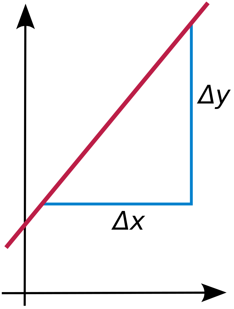
$y = 2x + 3$

$\frac{dy}{dx} = 2$

1.2 Non-Linear Functions

return to top

What if the Line is not Linear?

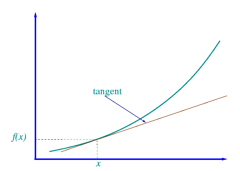
Use Differentiation to Find the Gradient at Point X

$y = x^2 + 20$

$\frac{dy}{dx} = 2x$

def func(x):
    return x**2 + 20

def gradient_at(x):
    return 2*x

x = np.array(list(range(50)))/10

fig = plt.figure(figsize=(12,6))
fig.add_subplot(111)


plt.subplot(1,2,1)
plt.title('Function', fontsize=20); plt.xlabel('x', fontsize=15); plt.ylabel('y', fontsize=15)
plt.plot(x, func(x), label='Function', c='r')
plt.subplot(1,2,2)
plt.title('Gradient', fontsize=20); plt.xlabel('x', fontsize=15); plt.ylabel('y', fontsize=15)
plt.plot(x, gradient_at(x), label='Gradient', c='g')
plt.show();

gradient_at(4)

8

1.3 Special Functions

return to top

Exponential Functions

$y = e^{2x}$

$\frac{dy}{dx} = 2e^{2x}$

def func(x):
    return np.exp(2*x)

def gradient_at(x):
    return 2 * np.exp(2*x)

x = np.array(list(range(50)))/10

fig = plt.figure(figsize=(12,6))
fig.add_subplot(111)

plt.subplot(1,2,1); plt.title('Function', fontsize=20); plt.xlabel('x', fontsize=15); plt.ylabel('y', fontsize=15)
plt.plot(x, func(x), label='Function', c='r')

plt.subplot(1,2,2); plt.title('Gradient', fontsize=20); plt.xlabel('x', fontsize=15); plt.ylabel('y', fontsize=15)
plt.plot(x, gradient_at(x),  label='Gradient', c='g')

plt.show();

Logarithmic Functions

$y = ln(5x)$

$\frac{dy}{dx} = \frac{1}{x}$

def func(x):
    return np.log(5*x)

def gradient_at(x):
    return 1/x

x = np.array(list(range(50)))/10 + 0.1

fig = plt.figure(figsize=(12,6))
fig.add_subplot(111)

plt.subplot(1,2,1)
plt.title('Function', fontsize=20); plt.xlabel('x', fontsize=15); plt.ylabel('y', fontsize=15)
plt.plot(x, func(x), label='Function', c='r')
plt.subplot(1,2,2)
plt.title('Gradient', fontsize=20); plt.xlabel('x', fontsize=15); plt.ylabel('y', fontsize=15)
plt.plot(x, gradient_at(x),  label='Gradient', c='g')
plt.show();

1.4 Gradients of Convex Functions

return to top

$y = x^2 - 9x + 25$

$\frac{dy}{dx} = 2x - 9$

def func(x):
    return x**2 - 9*x + 25

def gradient_at(x):
    return 2*x - 9

x = np.array(list(range(100)))/10

fig = plt.figure(figsize=(12,6))
fig.add_subplot(111)

plt.subplot(1,2,1); plt.axis([-0.5, 10.5, 0, 35])
plt.title('Function', fontsize=20); plt.xlabel('x', fontsize=15); plt.ylabel('y', fontsize=15)
plt.plot(x, func(x), label='Function', c='r')
plt.subplot(1,2,2)
plt.title('Gradient', fontsize=20); plt.xlabel('x', fontsize=15); plt.ylabel('y', fontsize=15)
plt.axhline(0, c='black', linewidth=0.5)
plt.plot(x, gradient_at(x),  label='Gradient', c='g')
plt.show();

gradient_at(5)

1

$\because 2x - 9 = Gradient$,

$x = \frac{Gradient + 9}{2}$

def find_x(gradient):
    return (gradient + 9)/2

At Minimum Point: $\frac{dy}{dx} = 0$

find_x(0)

4.5

x = np.array(list(range(100)))/10

fig = plt.figure(figsize=(12,6))
fig.add_subplot(111)

plt.subplot(1,2,1); plt.axis([-0.5, 10.5, 0, 35])
plt.title('Function', fontsize=20); plt.xlabel('x', fontsize=15); plt.ylabel('y', fontsize=15)
plt.plot(x, func(x), label='Function', c='r')
plt.axhline(func(find_x(0)), c='black', linestyle='--', linewidth=1)
plt.subplot(1,2,2)
plt.title('Gradient', fontsize=20); plt.xlabel('x', fontsize=15); plt.ylabel('y', fontsize=15)
plt.axhline(0, c='black', linewidth=0.5)
plt.plot(x, gradient_at(x),  label='Gradient', c='g')
plt.show();

# Minimum Point:
func(find_x(0))

4.75

1.5 Chain Rule in Differentiation

return to top

$y = 2x + 10$

$z = y - 3$

$a = z^2$

Therefore:

$a = (y-3)^2$

$a = ((2x + 10) - 3)^2$

What is $\frac{da}{dx}$?

$\frac{da}{dx} = \frac{da}{dz} \times \frac{dz}{dy} \times \frac{dy}{dx}$

$\frac{da}{dz} = 2z$

$\frac{dz}{dy} = 1$

$\frac{dy}{dx} = 2$

Therefore:

$\frac{da}{dx} = 2z \times 1 \times 2$

$\frac{da}{dx} = 4z = 4(y-3) = 4((2x + 10) - 3) = 4(2x + 7) = 8x + 28$

Key Point: We can solve for the Gradients of Nested Functions by Multiplying the Gradients Together

Practice Questions:

return to top

Question 1

$f(x) = 2x^2 + 4x$

Differentiate the Above Function with Respect to X

Question 2

$f(x, y) = 2x^2y + 4xy^3$

a) Differentiate the Above Function with Respect to X

b) Differentiate the Above Function with Respect to Y

Question 3

$y = 5x^2 + 2x$ $z = 2y^2 - 5$

Differentiate Z with Respect to X

Question 4

$y = x^2 - 9x + 25$

What is the Minimum Value of the Above Convex Function? (Find X and Y at the Minimum Point)

2) Gradients in Action

return to top

So why are Gradients so important in Machine Learning?

2.1 Cost Function

return to top

Recall our Problem from Earlier:

When trying to find the best estimate, we want to minimize the Error.

The Term "Cost Function" is used to represent the Total Error (Summation) for Each Datapoint.

We will see later on that, Cost Functions in most cases are Convex Functions

Which is to say, we can find the point of Minimum Error with Differentiation, by finding the point where the Gradients of the Cost Function with respect to each of the Parameters $\approx$ 0.

And to Differentiate the Error Function with respect to each Parameter, will require the application of the Chain Rule.

Consider "Mean Squared Error" as our Cost Function of a Linear Regression Model as a Nested Function:

$MSE = \frac{1}{m}\sum\limits^{m}_{i=1} (\hat{y} - y)^2$

$\hat{y} = w.x + b$

Where [w] and [b] are the Parameters to be Optimized

$\therefore \frac{dMSE}{dw} = \frac{dMSE}{d\hat{y}} \times \frac{d\hat{y}}{dw}$

$\therefore \frac{dMSE}{db} = \frac{dMSE}{d\hat{y}} \times \frac{d\hat{y}}{db}$

**The Chain can be Longer in More Complex Models

Goal: Find the Optimal Combination of [w] and [b] to achieve the Minimum Possible MSE

Therefore, we want both $\frac{dMSE}{dw}$ and $\frac{dMSE}{db}$ to $\approx$ 0

2.2 Gradient Descent

return to top

The Jacobian Matrix

The Jacobian Matrix is just a term for the Matrix of Gradients.

Jacobian Matrix $= \left[ {\begin{array}{c} \frac{dMSE}{dw} \\ \frac{dMSE}{db} \end{array} } \right] $

Plotting Our Cost Function against one of the Parameter

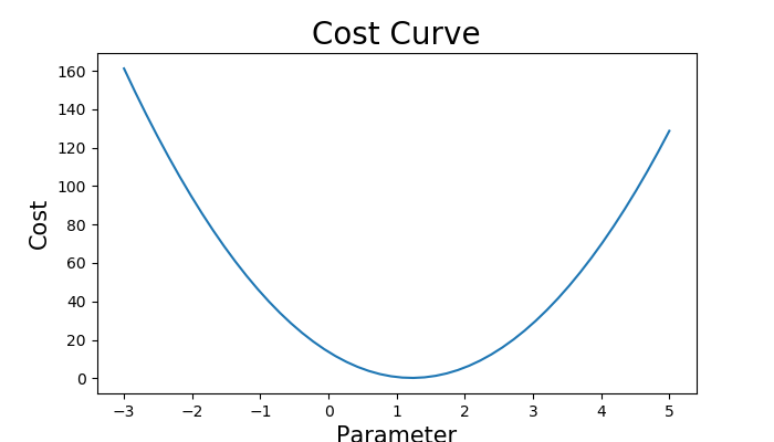
When the Parameter is too low, the Cost of our Model Increases.

When the Parameter is too high, the Cost of our Model Increases as well.

At Optimal Point of the Parameter, the Cost of our Model at Minimum

i.e. the Gradient is 0

**Take note that the Cost Curve is a Convex Function

How then, should we choose the weights for the Model?

Since we are doing Machine Learning, we can Randomly Initialize the weights and let the Machine Learn the Optimal Values of each Parameter.

We can adjust our randomly initialized Parameters towards the Optimal Point by utilizing the Jacobian Matrix (Gradients of Cost Curve with respect to each Parameter)

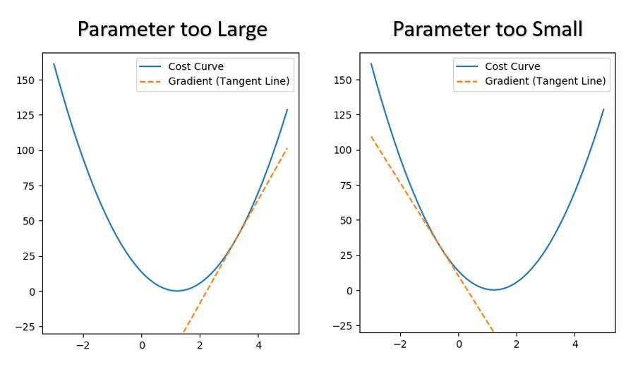
When the Parameter is too Large, the Gradient is POSITIVE, and we want to DECREASE the value of the Parameter.

When the Parameter is too Large, the Gradient is NEGATIVE. and we want to INCREASE the value of the Parameter.

Scenerio 1 - Parameter too Large:

• Gradient is POSITIVE

• Want to DECREASE the Value of the Parameter

Since we want to Decrease the value of the parameter, we can subtract a Positive Number from the Parameter.

Guess what Number is Positive??

Scenerio 2 - Parameter too Small:

• Gradient is NEGATIVE

• Want to INCREASE the Value of the Parameter

Since we want to Increase the value of the parameter, we can subtract a Negative Number from the Parameter.

Note: Subtracting a Negative Number is the same as Adding a Positive Number

Guess what Number is Negative??

Intuition:

If the Gradient is Positive, it means that the Parameter is too Large, and we can Reduce it by Subtracting the Positive Gradient.

If the Gradient is Negative, it means that the Parameter is too Small, and we can Increase it by Subtracting the Negative Gradient.

Therefore, Gradient Descent is Pretty Much:

$w := w - \frac{dMSE}{dw}$

$b := b - \frac{dMSE}{db}$

or

For Any Parameter:

$Param := Param - \frac{dMSE}{dParam}$

However, Gradients can be HUGE and it can throw the Parameters WAY OFF

Therefore, we scale the Gradient Down by a Small Number (Alpha)

A.K.A the Learning Rate, which is a Hyperparameter for the Training Algorithm

$w := w - \alpha\frac{dMSE}{dw}$

$b := b - \alpha\frac{dMSE}{db}$

or

For Any Parameter:

$Param := Param - \alpha\frac{dMSE}{dParam}$

With this, we are now ready to look at our First Example: Linear Regression

Previous: Next:

Intuition for Machine Learning (Part 1) Linear Regression