Machine Learning Programming Workshop

2.1 Linear Regression in Machine Learning

Prepared By: Cheong Shiu Hong (FTFNCE)

import numpy as np # Linear Algebra
import pandas as pd # Data Frames
import matplotlib.pyplot as plt # Visualization
import matplotlib.cm as cm # Color Mapping
from mpl_toolkits.mplot3d import axes3d # 3D Visualization
import ipywidgets as widgets # Interactivity
from IPython.display import display # Display Widgets

%matplotlib notebook

1) What is Linear Regression?

return to top

Best Fit Linear/Straight Line to Our Data

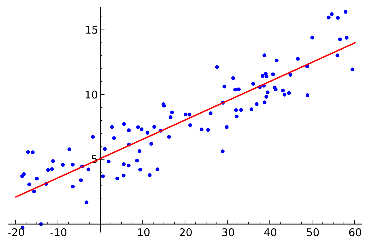
Gradient and Y-Intercept

Residuals/Error

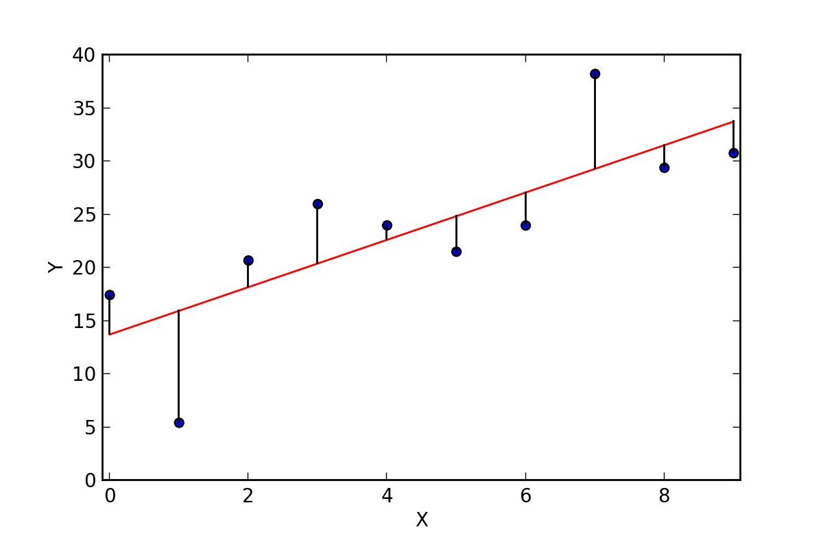
Goal: Minimize Sums of Squared Error for the Best Fit Line

We will:

- Use Vectors and Matrices to Represent Data

- Use Differentiation to Find Minimum SSE through Gradient Descent

Fake Dataset

x = np.array([1., 1.9, 1.2, 4., 3.2, 2.4, 3.6, 4.6])
y = np.array([1.5, 1.6, 1.4, 5.2, 4.5, 2.8, 3.9, 5.7 ])

pd.DataFrame({'x':x,'y':y})

fig = plt.figure(figsize=(4,3))
plt.scatter(x,y)
plt.show()

2) Model with 1 Parameter (Gradient Only)

return to top

$$\huge pred = b + w . x $$

$$$$

To Simplify, we set Y-Intercept (b) as Zero, Therefore:

$$$$$$\huge pred = w . x $$

def model(w, x):
    return w * x

def plot_model(title, init_weight=None):
    line_x = np.arange(-3, 8)
    if not init_weight:
        init_weight = np.random.randn(1)

    fig = plt.figure(figsize=(7,4))
    ax = fig.add_subplot(1,1,1)

    plt.suptitle('Model with 1 Variable', fontsize=15)
    plt.xlabel('X', fontsize=15)
    plt.ylabel('Y', fontsize=15)

    plt.axis([-4, 8, -4, 8])
    ax.axhline(0, color='black')
    ax.axvline(0, color='black')

    ax.scatter(x, y, c='red')
    line, = ax.plot(line_x, model(init_weight, line_x), c='green')

    def update(weight=init_weight):
        line.set_ydata(model(weight, line_x))
        fig.canvas.draw()

    gradient = widgets.FloatText(value=init_weight, description='Gradient', step=0.1)
    display(gradient)
    widgets.interactive(update, weight=gradient)

plot_model('Model with 1 Variable')

2.1 Cost Function (Mean Squred Error)

return to top

$$Cost(MSE) = \frac{1}{m}\sum\limits_{i=1}^{m}(\hat{y_{i}} - y_{i})^2$$

Where

$$\huge \hat{y_{i}} = w . x_{i}$$

Therefore$$ Cost(MSE) = \frac{1}{m}\sum\limits_{i=1}^{m}((w.x_{i}) - y_{i})^2$$

2.2 Simulation for Visualization

return to top

Create Simulation Data for Each Possible Point of [w]

size = 50

w_sim = np.linspace(-3, 5, size)

w_matrix = w_sim.reshape(size, 1)
x_matrix = x.reshape(1, x.shape[0])
y_matrix = y.reshape(1, y.shape[0])

pred_sim = w_matrix * x_matrix
error_sim = (pred_sim - y_matrix)
cost_sim = np.sum(error_sim**2, 1)/len(y)

w_sim

array([-3.        , -2.83673469, -2.67346939, -2.51020408, -2.34693878,
       -2.18367347, -2.02040816, -1.85714286, -1.69387755, -1.53061224,
       -1.36734694, -1.20408163, -1.04081633, -0.87755102, -0.71428571,
       -0.55102041, -0.3877551 , -0.2244898 , -0.06122449,  0.10204082,
        0.26530612,  0.42857143,  0.59183673,  0.75510204,  0.91836735,
        1.08163265,  1.24489796,  1.40816327,  1.57142857,  1.73469388,
        1.89795918,  2.06122449,  2.2244898 ,  2.3877551 ,  2.55102041,
        2.71428571,  2.87755102,  3.04081633,  3.20408163,  3.36734694,
        3.53061224,  3.69387755,  3.85714286,  4.02040816,  4.18367347,
        4.34693878,  4.51020408,  4.67346939,  4.83673469,  5.        ])

cost_sim

array([161.19125   , 148.98641035, 137.26250364, 126.01952988,
       115.25748907, 104.9763812 ,  95.17620627,  85.85696429,
        77.01865525,  68.66127915,  60.78483601,  53.3893258 ,
        46.47474854,  40.04110423,  34.08839286,  28.61661443,
        23.62576895,  19.11585641,  15.08687682,  11.53883017,
         8.47171647,   5.88553571,   3.7802879 ,   2.15597303,
         1.01259111,   0.35014213,   0.16862609,   0.468043  ,
         1.24839286,   2.50967566,   4.2518914 ,   6.47504009,
         9.17912172,  12.3641363 ,  16.03008382,  20.17696429,
        24.8047777 ,  29.91352405,  35.50320335,  41.5738156 ,
        48.12536079,  55.15783892,  62.67125   ,  70.66559402,
        79.14087099,  88.0970809 ,  97.53422376, 107.45229956,
       117.85130831, 128.73125   ])

Visualization of Cost Curve

fig = plt.figure(figsize=(7,4))
ax = fig.add_subplot(111)

plt.title('Cost Curve', fontsize=20)
ax.set_xlabel('Parameter', fontsize=15)
ax.set_ylabel('Cost', fontsize=15)

ax.plot(w_sim, cost_sim)
plt.show()

Calling out Minimum Point from Simulation

minimum_cost_index = np.argmin(cost_sim)
best_w = w_sim[minimum_cost_index]
print('Minimum Index:', minimum_cost_index, \
      '\nCost:', cost_sim[minimum_cost_index], \
      '\nGradient:', w_sim[minimum_cost_index])

Minimum Index: 26 
Cost: 0.16862609329446043 
Gradient: 1.2448979591836729

plot_model('Model with Best Weight', init_weight=best_w)

2.3 Derivative of Cost Function

return to top

How can we fit a linear regression line without simulation?

1) Formula:

$$ w = \frac{\sum\limits_{i=1}^{m}(x_i-\bar{x})(y_i-\bar{y})}{\sum\limits_{i=1}^{m}(x_i-\bar{x})^2}$$

$$ b = \bar{y} - w.\bar{x}$$

What about Multiple Regression, when there are 3 or more Coefficients to be optimized?

2) Mathematical Optimization with Gradients

$$ \frac{dCost}{dW} = \frac{dCost}{dError} \times \frac{dError}{d\hat{y}} \times \frac{d\hat{y}}{dW} $$

$$$$

x = Input Data (Independent Variable)

w = Weights to be Optimized

y = True Values of Each Input Data (Dependent Variable)

$$$$

$\hat{y} = w . x$

$error = \hat{y} - y$

$cost = error^2$

$$$$

Derivatives:

Find $\frac{dCost}{dW}$:

$$$$

$\frac{dCost}{dError} = 2 \times error$

$\frac{dError}{d\hat{y}} = 1$

$\frac{dPred}{dW} = x$

$$$$

$\frac{dCost}{dW} = \frac{dCost}{dError} \times \frac{dError}{d\hat{y}} \times \frac{dPred}{dW}$

$\frac{dCost}{dW} = (2 \times error) \times (1) \times (x)$

$\frac{dCost}{dW} = 2x \times error$

$\frac{dCost}{dW} = 2x \times (pred - y)$

$\frac{dCost}{dW} = 2x \times ((w . x) - y)$

What about Normal Equations?

Normal Equations would be more effecient for a simple task, but in high dimensionality problems, gradient descent would be more efficient.

2.4 Demonstration of Gradient Descent

return to top

def one_iteration(x, y, learning_rate=1e-2, first=False):
    global theta, prev_theta
    prev_theta = theta
    
    # Model
    pred = np.dot(theta, x)
    
    # Calculations for Backpropagation
    error = pred - y # Error
    cost = sum(error**2)/len(error) # Cost
    dcost_dtheta = sum(2 * x * error)/len(error) # Gradient of Weight
    theta = theta - (dcost_dtheta * learning_rate) # Update Weight
    
    data = "Cost: {}\nWeight: {}\nGradient of Cost Curve: {}\n".format(cost, theta, dcost_dtheta)
    
    return cost, dcost_dtheta, data

def update(iterations):
    global x, y, theta, w_sim, intercept, out
    cost, dcost_dtheta, data = one_iteration(x, y)
    intercept = cost - (prev_theta * dcost_dtheta)
    tangent.set_ydata((dcost_dtheta * w_sim) + intercept)
    line.set_ydata(model(theta, line_x))
    out.clear_output()
    fig.canvas.draw()
    out.append_stdout(data)

def update_ten(iterations):
    for i in range(10):
        update(1)

##### Widgets #####
out = widgets.Output(layout={'border': '1px solid black'})      
button_one = widgets.Button(description="1 Iteration")
button_one.on_click(update)
button_ten = widgets.Button(description="10 Iterations")
button_ten.on_click(update_ten)
hbox = widgets.HBox([button_one, button_ten])

# Initialize Random Weight
theta = np.random.uniform(-2,4)

##### Plot #####
fig = plt.figure(figsize=(10,5))
ax = fig.add_subplot(111)

plt.suptitle('Cost Curve & Regression Line Plot', fontsize=20)
ax.set_xlabel('Gradient', fontsize=15)
ax.set_ylabel('Cost', fontsize=15)

# Plot 1
plt.subplot(1,2,1)
##### Cost Curve #####
plt.plot(w_sim, cost_sim, label='Cost Curve')
x1,x2,y1,y2 = plt.axis()
plt.axis((x1,x2,-30,y2))
##### Tangent #####
cost, dcost_dtheta, data = one_iteration(x, y)
intercept = cost - (prev_theta * dcost_dtheta)
tangent, = plt.plot(w_sim, (dcost_dtheta * w_sim) + intercept, label='Gradient (Tangent Line)', linestyle='--')
plt.legend();

# Plot 2
plt.subplot(1,2,2)
plt.axis([-2,8,-2,10])
plt.axhline(0, color='black')
plt.axvline(0, color='black')
line_x = np.arange(-3, 8)
##### Data Points #####
plt.scatter(x, y, c='red', label='True')
##### Regression #####
line, = plt.plot(line_x, model(theta, line_x), c='green', label='Line')
plt.legend();

update(1)
display(hbox, out)

3) Model with 2 Parameters (Gradient and Y-Intercept)

return to top

$$\huge pred = b + w . x $$$$$$

Expressed as:

$$$$ $$\huge pred = \theta_0 + \theta_1 . x$$

def model(b, w, x):
    return b + w * x

def plot_model(title, init_weight=None, init_bias=None):
    line_x = np.arange(-3, 8)
    if not init_weight:
        init_weight = np.random.randn(1)
    if not init_bias:
        init_bias = np.random.randn(1)

    fig = plt.figure(figsize=(7,4))
    ax = fig.add_subplot(1,1,1)

    plt.suptitle(title, fontsize=15)
    plt.xlabel('X', fontsize=15)
    plt.ylabel('Y', fontsize=15)

    plt.axis([-4, 8, -4, 8])
    ax.axhline(0, color='black')
    ax.axvline(0, color='black')

    ax.scatter(x, y, c='red')
    line, = ax.plot(line_x, model(init_bias, init_weight, line_x), c='green')

    def update(weight=init_weight, intercept=init_bias):
        line.set_ydata(model(intercept, weight, line_x))
        fig.canvas.draw()

    gradient = widgets.FloatText(value=init_weight, description='Gradient', step=0.2)
    intercept = widgets.FloatText(value=init_bias, description='Y-Intercept', step=0.2)
    display(gradient, intercept)
    widgets.interactive(update, weight=gradient, intercept=intercept)

plot_model('Model with 2 Variables')

3.1 Simulation for Visualization

Create Simulation Data for Each Possible Point of $\theta_0$ and $\theta_1$

return to top

size = 50 # Number of Simulated Points

w_sim = np.linspace(-5, 5, size) # x Size Linearly Spaced Points Between -10 and 10
b_sim = np.linspace(-5, 5, size)
W, B = np.meshgrid(w_sim, b_sim)

w_matrix = w_sim.reshape(size, 1)
b_matrix = b_sim.reshape(1, size)
x_matrix = x.reshape(1, x.shape[0])
y_matrix = y.reshape(1, y.shape[0])

# (Sw,1) x (1xN) --> (Sw,N) --reshape--> (Sw,N,1)
wx = (w_matrix * x_matrix).reshape(size, x.shape[0], 1) 

# (Sw,N,1) + (1,Sb) --> (Sw,N,Sb) --tranpose--> (Sw,Sb,N)
pred_sim = (wx + b_matrix).transpose(0, 2, 1) 

# ((Sw,Sb,N) - (1,N))^2 --> (Sw,Sb,N)
error_sim = pred_sim - y_matrix
squared_error_sim = error_sim**2 

# Flatten (Sw,Sb) --> (Sw x Sb)
cost_sim = squared_error_sim.sum(-1)/len(y) # Sum (50, 50, 8) in Dim 2 --> (50, 50)

# For Calling Out
plot_cost = cost_sim.reshape(-1) # Flatten (50,50) --> (2500,)
plot_w = np.repeat(w_sim, size)
plot_b = np.tile(b_sim, size)

# 3D Visualization
fig = plt.figure(figsize=(9,5))
ax = fig.add_subplot(111, projection='3d')

plot = ax.plot_surface(W, B, cost_sim, cmap=cm.nipy_spectral)#, color=plot_cost, cmap='nipy_spectral')

cbar=plt.colorbar(plot)
cbar.set_label('\nCost', fontsize=20)

plt.title('Cost Curve\n', fontsize=20)
ax.set_xlabel('Gradient', fontsize=15)
ax.set_ylabel('Y-Intercept', fontsize=15)
ax.set_zlabel(' Cost', fontsize=15)

plt.show()

minimum_cost_index = np.argmin(plot_cost)
best_w = plot_w[minimum_cost_index]
best_b = plot_b[minimum_cost_index]
print('Minimum Index:', minimum_cost_index, \
      '\nCost:', plot_cost[minimum_cost_index], \
      '\nY-Intercept:', plot_b[minimum_cost_index], \
      '\nGradient:', plot_w[minimum_cost_index])

Minimum Index: 1573 
Cost: 0.164350791336943 
Y-Intercept: -0.3061224489795915 
Gradient: 1.3265306122448983

plot_model('Model with 2 Variables', init_weight=best_w, init_bias=best_b)

Verify with Normal Equation

xbar = x.mean() 
ybar = y.mean()

normal_w = ((x - xbar)*(y - ybar)).sum() / ((x - xbar)**2).sum()
normal_b = ybar - normal_w * xbar

print(normal_w, normal_b)

1.2752941176470587 -0.16611764705882326

3.2) Derivatives of Cost Function

return to top

$$ Pred = \theta_0 + \theta_1.x $$

$$ Error = Pred - y $$

$$ Cost = Error^2 $$

$$ \frac{dCost}{d\theta_0} = \frac{dCost}{dError} \times \frac{dError}{dPred} \times \frac{dPred}{d\theta_0} $$ $$$$ $$ \frac{dCost}{d\theta_1} = \frac{dCost}{dError} \times \frac{dError}{dPred} \times \frac{dPred}{d\theta_1} $$

x = Input Data (Independent Variable)

$\theta$ = Weights to be Optimized

y = True Values of Each Input Data (Dependent Variable)

$pred = \theta_0 + (\theta_1 . x) $

$error = pred - y$

$cost = error^2$

Derivatives:

Find $\frac{dCost}{d\theta_0} and \frac{dCost}{d\theta_1}$

Recap: $\frac{dCost}{d\theta_1} = 2x \times (\theta_0 + (\theta_1.x) - y)$

$\frac{dCost}{dError} = 2 \times error$

$\frac{dError}{dPred} = 1$

$\frac{dPred}{d\theta_0} = 1$

$\frac{dCost}{d\theta_0} = \frac{dCost}{dError} \times \frac{dError}{dPred} \times \frac{dPred}{d\theta_0}$

$\frac{dCost}{d\theta_0} = (2 \times error) \times (1) \times (1)$

$\frac{dCost}{d\theta_0} = 2 \times error$

$\frac{dCost}{d\theta_0} = 2 \times (pred - y)$

$\frac{dCost}{d\theta_0} = 2 \times (\theta_0 + (\theta_1.x)) - y)$

3.3 Demonstration of Gradient Descent

return to top

def one_iteration(x, y, learning_rate=1e-2, first=False):
    global theta, prev_theta
    prev_theta = theta
    
    X = np.vstack([np.ones(y.shape[0]), x])

    # Model
    pred = np.dot(theta, X)
    
    # Calculations for Backpropagation
    error = pred - y
    cost = sum(error**2)/len(error)
    dcost_dtheta = np.array([sum(2 * Xi * error)/len(error) for Xi in X])
    theta = theta - (dcost_dtheta * learning_rate)
    
    if len(x.shape) == 1:
        data = "Cost: {}\nBias: {}\nWeight: {}\nGradient of Cost Curve to Bias: {}\
            \nGradient of Cost Curve to Weight: {}\n".format(cost, theta[0], theta[1], dcost_dtheta[0], dcost_dtheta[1])
    elif len(x.shape) == 2:
        data = "Cost: {}\nBias: {}\nWeight 1: {}\nWeight 2: {}\nGradient of Cost Curve to Bias: {}\
            \nGradient of Cost Curve to Weight 1: {}\nGradient of Cost Curve to Weight 2: {}\n"\
            .format(cost, theta[0], theta[1], theta[2], dcost_dtheta[0], dcost_dtheta[1], dcost_dtheta[2])
    
    return cost, dcost_dtheta, data

def find_nearest(array, value):
    idx = (np.abs(array - value)).argmin()
    return idx

def update(iterations, nested=0):
    # Run Iteration
    if nested:
        for i in range(nested):
            cost, dcost_dtheta, data = one_iteration(x, y)
    else:
        cost, dcost_dtheta, data = one_iteration(x, y)
    # Replot Cost Curves
    b_nearest = find_nearest(b_sim, prev_theta[0])
    w_nearest = find_nearest(w_sim, prev_theta[1])
    curve_b.set_ydata(cost_sim[w_nearest])
    curve_w.set_ydata(cost_sim[:, b_nearest])
    # Replot Tangents
    intercept_b = cost - (prev_theta[0] * dcost_dtheta[0])
    intercept_w = cost - (prev_theta[1] * dcost_dtheta[1])
    tangent_b.set_ydata((dcost_dtheta[0]*b_sim)+intercept_b)
    tangent_w.set_ydata((dcost_dtheta[1]*w_sim)+intercept_w)
    # Replot Regression Line
    line.set_ydata(model(theta[0], theta[1], line_x))
    # Clear and Redraw
    out.clear_output()
    fig.canvas.draw()
    out.append_stdout(data)

def update_ten(iterations):
    if visualize.value:
        for i in range(10):
            update(1)
    else:
        update(1, nested=10)

def update_hundred(iterations):
    if visualize.value:
        for i in range(100):
            update(1)
    else:
        update(1, nested=100)

##### Widgets #####
out = widgets.Output(layout={'border': '1px solid black'})
button_one = widgets.Button(description="1 Iteration")
button_one.on_click(update)
button_ten = widgets.Button(description="10 Iterations")
button_ten.on_click(update_ten)
button_hundred = widgets.Button(description="!!!100 Iterations!!!")
button_hundred.on_click(update_hundred)
visualize = widgets.Checkbox(value=True, description='Visualize Changes', disabled=False)
hbox = widgets.HBox([button_one, button_ten, button_hundred, visualize])

# Initialize Random Weight & Bias
theta = np.random.uniform(-8,8, size=2)
# theta = np.array([-5, 5])

# Run First Iteration
cost, dcost_dtheta, data = one_iteration(x, y)

b_nearest = find_nearest(b_sim, theta[0])
w_nearest = find_nearest(w_sim, theta[1])

############################
### Visualize Cost Curve ###
############################
fig = plt.figure(figsize=(9,6))
ax = fig.add_subplot(111)
plt.suptitle('Cost Curves')

##### Bias Subplot #####
plt.subplot(2,2,1)
# plt.axis([-10.5,10.5,-500,2000])
plt.title('Bias')
plt.xlabel('Bias')
plt.ylabel('Cost')
# Cost Curve
curve_b, = plt.plot(b_sim, cost_sim[w_nearest], label='Cost Curve')
x1, x2, y1, y2 = plt.axis()
plt.axis([x1,x2,-100,y2])
# Tangent
intercept_b = cost - (prev_theta[0] * dcost_dtheta[0])
tangent_b, = plt.plot(b_sim, (dcost_dtheta[0]*b_sim)+intercept_b, label='Gradient (Tangent Line)', linestyle='--')
plt.legend();

##### Weight Subplot #####
plt.subplot(2,2,2)
plt.title('Weight')
plt.xlabel('Weight')
# Cost Curve
curve_w, = plt.plot(w_sim, cost_sim[:, b_nearest], label='Cost Curve')
x1, x2, y1, y2 = plt.axis()
plt.axis([x1,x2,-300,y2])
# Tangent
intercept_w = cost - (prev_theta[1] * dcost_dtheta[1])
tangent_w, = plt.plot(w_sim, (dcost_dtheta[1]*w_sim)+intercept_w, label='Gradient (Tangent Line)', linestyle='--')
plt.legend();

##### Regression Line Subplot #####
plt.subplot(2,2,(3,4))
plt.axis([-1,8,-3,10])
plt.title('Regression')
plt.xlabel('X', fontsize=15)
plt.ylabel('Y', fontsize=15)
plt.axhline(0, color='black')
plt.axvline(0, color='black')
line_x = np.arange(-3, 8)
##### Data Points #####
plt.scatter(x, y, label='True Values', c='red')
##### Regression #####
line, = plt.plot(line_x, model(theta[0], theta[1], line_x), label='Regression Line', c='green')
plt.legend();

update(1)
display(hbox)   
out

4) Model with Three Parameters (Multiple Regression)

$$\huge pred = b + w_1.x_1 + w_2.x_2 $$ $$$$

Expressed as:

$$$$ $$\huge pred = \theta_0 + \theta_1 . x_1 + \theta_2 . x_2$$

return to top

def model(b, w1, x1, w2, x2):
    return b + (w1 * x1) + (w2 * x2)

New Fake Data for Multiple Regression

x1 = np.array([1., 1.9, 1.2, 4., 3.2, 2.4, 3.6, 4.6])
x2 = np.array([8.1, 6.7, 6.5, 3.2, 3.4, 6.6, 3.9, 3.5])
y = np.array([1.5, 1.6, 1.4, 5.2, 4.5, 2.8, 3.9, 5.7 ])

X = np.vstack([x1, x2])

fig = plt.figure(figsize=(5,4))
plt.title('x1 vs Y'); plt.xlabel('x1'); plt.ylabel('Y')
plt.scatter(x1, y, c='r')
plt.show()

fig = plt.figure(figsize=(5,4))
plt.title('x2 vs Y'); plt.xlabel('x2'); plt.ylabel('Y')
plt.scatter(x2, y, c='g')
plt.show()

line_x1 = np.linspace(0, 10, size)
line_x2 = np.linspace(0, 10, size)
lx1, lx2 = np.meshgrid(line_x1, line_x2)
init = np.random.randn(3)

fig = plt.figure(figsize=(8,5))
ax = fig.add_subplot(111, projection='3d')

ax.scatter(x1, x2, y, s=100, c='r')
z = model(init[0], init[1], lx1, init[2], lx2)
ax.plot_surface(lx1, lx2, z, color='green', alpha=0.5)

plt.suptitle('Model with 3 Variables', fontsize=15)

plt.axes([0, 10, 0, 10])

def update(intercept=init[0], weight_1=init[1], weight_2=init[2]):
    global ax, line
    ax.clear()
    ax.set_xlabel('X1', fontsize=15)
    ax.set_ylabel('X2', fontsize=15)
    ax.set_zlabel('Y', fontsize=15)
    ax.scatter(x1, x2, y, s=100, c='r')
    z = model(intercept, weight_1, lx1, weight_2, lx2)
    line = ax.plot_surface(lx1, lx2, z, color='green', alpha=0.5)
    fig.canvas.draw()
    
intercept = widgets.FloatText(value=init[0], description='Y-Intercept')
gradient_1 = widgets.FloatText(value=init[1], description='Gradient 1')
gradient_2 = widgets.FloatText(value=init[2], description='Gradient 2')

widgets.interactive(update, intercept=intercept, weight_1=gradient_1, weight_2=gradient_2)

4.1 Simulation for Visualization

Create Simulation Data for Each Possible Point of $\theta_0$, $\theta_1$, and $\theta_2$

return to top

size = 20

w1_raw = np.linspace(-5,5,size)
w2_raw = np.linspace(-5,5,size)

w1_sim = np.repeat(w1_raw, size)
w2_sim = np.tile(w2_raw, size)
b_sim = np.linspace(-10, 10, size)

w1_matrix = w1_sim.reshape(size*size, 1)
w2_matrix = w2_sim.reshape(size*size, 1)
b_matrix = b_sim.reshape(1, size)
x1_matrix = x1.reshape(1, x1.shape[0])
x2_matrix = x2.reshape(1, x2.shape[0])
y_matrix = y.reshape(1, y.shape[0])

# (Sw2xSw1,1) x (1xN) --> (Sw2xSw1,N) --reshape--> (Sw1xSw2,N,1)
w_matrix = np.hstack([w1_matrix, w2_matrix])
x_matrix = np.vstack([x1_matrix, x2_matrix])
wx = np.dot(w_matrix, x_matrix).reshape(size*size, x1.shape[0], 1)

# (Sw2xSw1,N,1) + (1,Sb) --> (Sw2xSw1,N,Sb) --tranpose--> (Sw2xSw1,Sb,N)
pred_sim = (wx + b_matrix).transpose(0, 2, 1) 

# ((Sw1xSw2,Sb,N) - (1,N))^2 --> (Sw1xSw2,Sb,N)
error_sim = pred_sim - y_matrix
squared_error_sim = error_sim**2 

# Sum (Sw1xSw2,Sb,N) in Dim 2 --> (Sw1xSw2,Sb)
cost_sim = np.sum(squared_error_sim, len(squared_error_sim.shape)-1)/len(y)

# Flatten (Sw1xSw2,Sb) --> (Sw1xSw2 x Sb)
plot_cost = cost_sim.reshape(-1) # Flatten (50,50) --> (2500,)

plot_w1 = np.repeat(w1_raw, size*size)
plot_w2 = np.tile(np.repeat(w2_raw, size), size)
plot_b = np.tile(b_sim, size*size)

pd.DataFrame({'Gradient_1': plot_w1, 'Gradient_2': plot_w2, 'Intercept': plot_b, 'Cost': plot_cost}).head(5)

# 3D Visualization
fig = plt.figure(figsize=(8,5))
ax = fig.add_subplot(111, projection='3d')

plot = ax.scatter(plot_w1, plot_w2, plot_b, c=plot_cost, cmap='nipy_spectral')

cbar=plt.colorbar(plot)
cbar.set_label('\nCost', fontsize=20)

plt.title('Cost Curve\n', fontsize=30)
ax.set_xlabel('Gradient 1 (Theta 1)', fontsize=15)
ax.set_ylabel('Gradient 2 (Theta 2)', fontsize=15)
ax.set_zlabel(' Y-Intercept (Theta 0)', fontsize=15)

plt.show()

minimum_cost_index = np.argmin(plot_cost)
best_b = plot_b[minimum_cost_index]
best_w1 = plot_w1[minimum_cost_index]
best_w2 = plot_w2[minimum_cost_index]
print('Minimum Index:', minimum_cost_index, \
      '\nCost:', plot_cost[minimum_cost_index], \
      '\nY-Intercept:', plot_b[minimum_cost_index], \
      '\nGradient 1:', plot_w1[minimum_cost_index], \
      '\nGradient 2:', plot_w2[minimum_cost_index])

Minimum Index: 4592 
Cost: 0.17524238227146763 
Y-Intercept: 2.6315789473684212 
Gradient 1: 0.7894736842105257 
Gradient 2: -0.2631578947368425

fig = plt.figure(figsize=(8,5))
ax = fig.add_subplot(111, projection='3d')

ax.scatter(x1, x2, y, s=100, c='r')
z = model(best_b, best_w1, lx1, best_w2, lx2)
ax.plot_surface(lx1, lx2, z, color='green', alpha=0.5)

plt.suptitle('Model with 3 Variables', fontsize=15)

plt.axes([0, 10, 0, 10])

def update(intercept=best_b, weight_1=best_w1, weight_2=best_w2):
    global ax, line
    ax.clear()
    ax.set_xlabel('X1', fontsize=15)
    ax.set_ylabel('X2', fontsize=15)
    ax.set_zlabel('Y', fontsize=15)
    ax.scatter(x1, x2, y, s=100, c='r')
    z = model(intercept, weight_1, lx1, weight_2, lx2)
    line = ax.plot_surface(lx1, lx2, z, color='green', alpha=0.5)
    fig.canvas.draw()
    
intercept = widgets.FloatText(value=best_b, description='Y-Intercept')
gradient_1 = widgets.FloatText(value=best_w1, description='Gradient 1')
gradient_2 = widgets.FloatText(value=best_w2, description='Gradient 2')

widgets.interactive(update, intercept=intercept, weight_1=gradient_1, weight_2=gradient_2)

4.2 Derivatives of Cost Function

return to top

$$ Pred = \theta_0 + \theta_1.x_1 + \theta_2.x_2 $$

$$ Error = Pred - y $$

$$ Cost = Error^2 $$

$$ \frac{Cost}{d\theta_0} = \frac{dCost}{dError} \times \frac{dError}{dPred} \times \frac{dPred}{d\theta_0} $$ $$$$ $$ \frac{dCost}{d\theta_1} = \frac{dCost}{dError} \times \frac{dError}{dPred} \times \frac{dPred}{d\theta_1} $$ $$$$ $$ \frac{dCost}{d\theta_2} = \frac{dCost}{dError} \times \frac{dError}{dPred} \times \frac{dPred}{d\theta_2} $$

x = Input Data (Independent Variable)

w = Weights to be Optimized

y = True Values of Each Input Data (Dependent Variable)

$pred = \theta_0 + (\theta_1 . x_1) + (\theta_2 . x2)$

$error = pred - y$

$cost = error^2$

Derivatives:

Find $\frac{dCost}{d\theta_0}, \frac{dCost}{d\theta_1}, and \frac{dCost}{d\theta_2}$

Recap: $\frac{dCost}{d\theta_0} = 2 \times (\theta_0 + (\theta_1.x_1) + (\theta_2.x_2) - y)$

Recap: $\frac{dCost}{d\theta_1} = 2x_1 \times (\theta_0 + (\theta_1.x_1) + (\theta_2.x_2) - y)$

$\frac{dCost}{dError} = 2 \times error$

$\frac{dError}{dPred} = 1$

$\frac{dPred}{d\theta_2} = x_2$

$\frac{dCost}{d\theta_2} = \frac{dCost}{dError} \times \frac{dError}{dPred} \times \frac{dPred}{d\theta_2}$

$\frac{dCost}{d\theta_2} = (2 \times error) \times (1) \times (x_2)$

$\frac{dCost}{d\theta_2} = 2x_2 \times error$

$\frac{dCost}{d\theta_2} = 2x_2 \times (pred - y)$

$\frac{dCost}{d\theta_2} = 2x_2 \times (\theta_0 + (\theta_1.x_1) + (\theta_2.x_2) - y)$

Therefore:

$\frac{dCost}{d\theta_0} = 2 \times (\theta_0 + (\theta_1.x_1) + (\theta_2.x_2) - y)$

$\frac{dCost}{d\theta_1} = 2x_1 \times (\theta_0 + (\theta_1.x_1) + (\theta_2.x_2) - y)$

$\frac{dCost}{d\theta_2} = 2x_2 \times (\theta_0 + (\theta_1.x_1) + (\theta_2.x_2) - y)$

4.3 Demonstration of Gradient Descent

return to top

def find_nearest(array, value):
    idx = (np.abs(array - value)).argmin()
    return idx

def match(array, value):
    cond = array == value
    return np.where(cond)[0]

def match_2(array1, array2, value1, value2):
    cond1 = array1 == value1
    cond2 = array2 == value2
    a = np.where(cond1)[0]
    b = np.where(cond2)[0]
    return a[np.where(np.in1d(a, b))][0]
    
def update(iterations, nested=0):
    # Run Iteration
    if nested:
        for i in range(nested):
            cost, dcost_dtheta, data = one_iteration(X, y)
    else:
        cost, dcost_dtheta, data = one_iteration(X, y)
    # Replot Cost Curves
    b_nearest = find_nearest(b_sim, prev_theta[0])
    w1_nearest = find_nearest(w1_raw, prev_theta[1])
    w2_nearest = find_nearest(w2_raw, prev_theta[2])
    curve_b.set_ydata(cost_sim[match_2(w1_sim, w2_sim, w1_raw[w1_nearest], w2_raw[w2_nearest])])
    curve_w1.set_ydata(cost_sim[match(w2_sim, w2_raw[w2_nearest]), b_nearest])
    curve_w2.set_ydata(cost_sim[match(w1_sim, w1_raw[w1_nearest]), b_nearest])
    # Replot Tangents
    intercept_b = cost - (prev_theta[0] * dcost_dtheta[0])
    intercept_w1 = cost - (prev_theta[1] * dcost_dtheta[1])
    intercept_w2 = cost - (prev_theta[2] * dcost_dtheta[2])
    tangent_b.set_ydata((dcost_dtheta[0]*b_sim)+intercept_b)
    tangent_w1.set_ydata((dcost_dtheta[1]*w1_raw)+intercept_w1)
    tangent_w2.set_ydata((dcost_dtheta[2]*w2_raw)+intercept_w2)
    # Clear and Redraw
    out.clear_output()
    out.append_stdout(data)
    fig.canvas.draw()

def update_ten(iterations):
    if visualize.value:
        for i in range(10):
            update(1)
    else:
        update(1, nested=10)

def update_hundred(iterations):
    if visualize.value:
        for i in range(100):
            update(1)
    else:
        update(1, nested=100)
        
def update_thousand(iterations):
    if visualize.value:
        print('Not Allowed, Unselect Visualize to Proceed.')
    else:
        update(1, nested=1000)
        
##### Widgets #####
out = widgets.Output(layout={'border': '1px solid black'})
button_one = widgets.Button(description="1 Iteration")
button_one.on_click(update)
button_ten = widgets.Button(description="10 Iterations")
button_ten.on_click(update_ten)
button_hundred = widgets.Button(description="!!!100 Iterations!!!")
button_hundred.on_click(update_hundred)
button_thousand = widgets.Button(description="!!!Warning - 1000!!!")
button_thousand.on_click(update_thousand)
visualize = widgets.Checkbox(value=True, description='Visualize Changes', disabled=False)
hbox = widgets.HBox([button_one, button_ten, button_hundred, button_thousand, visualize])

# Initialize Random Weights & Bias
theta = np.random.uniform(-5,5,size=3)

# Run First Iteration
cost, dcost_dtheta, data = one_iteration(X, y)
                           
b_nearest = find_nearest(b_sim, prev_theta[0])
w1_nearest = find_nearest(w1_raw, prev_theta[1])
w2_nearest = find_nearest(w2_raw, prev_theta[2])

############################
### Visualize Cost Curve ###
############################
fig = plt.figure(figsize=(10.5,5))
ax = fig.add_subplot(111)
plt.suptitle('Cost Curves')

##### Bias Subplot #####
plt.subplot(1,3,1)
plt.title('Bias')
plt.xlabel('Bias')
plt.ylabel('Cost')
# Cost Curve
curve_b, = plt.plot(b_sim, cost_sim[match_2(w1_sim, w2_sim, w1_raw[w1_nearest], w2_raw[w2_nearest])], label='Cost Curve')
d1,d2,d3,d4 = plt.axis()
plt.axis([d1,d2,-50,200])
# Tangent
intercept_b = cost - (prev_theta[0] * dcost_dtheta[0])
tangent_b, = plt.plot(b_sim, (dcost_dtheta[0]*b_sim)+intercept_b, label='Gradient (Tangent Line)', linestyle='--')
plt.legend();

##### Weight 1 Subplot #####
plt.subplot(1,3,2)
# plt.axis([-30.5,30.5,-1000,1000])
plt.title('Weight 1')
plt.xlabel('Weight 1')
# Cost Curve
curve_w1, = plt.plot(w1_raw, cost_sim[match(w2_sim, w2_raw[w2_nearest]), b_nearest], label='Cost Curve')
d1,d2,d3,d4 = plt.axis()
plt.axis([d1,d2,-100,1200])
# Tangent
intercept_w1 = cost - (prev_theta[1] * dcost_dtheta[1])
tangent_w1, = plt.plot(w1_raw, (dcost_dtheta[1]*w1_raw)+intercept_w1, label='Gradient (Tangent Line)', linestyle='--')
plt.legend();

##### Weight 2 Subplot #####
plt.subplot(1,3,3)
plt.title('Weight 2')
plt.xlabel('Weight 2')
# Cost Curve
curve_w2, = plt.plot(w2_raw, cost_sim[match(w1_sim, w1_raw[w1_nearest]), b_nearest], label='Cost Curve')
d1,d2,d3,d4 = plt.axis()
plt.axis([d1,d2,-300,3500])
# Tangent
intercept_w2 = cost - (prev_theta[2] * dcost_dtheta[2])
tangent_w2, = plt.plot(w2_raw, (dcost_dtheta[2]*w2_raw)+intercept_w2, label='Gradient (Tangent Line)', linestyle='--')
plt.legend();

update(1)
display(hbox)   
out

def update(iterations, nested=0):
    cost, dcost_dtheta, data = one_iteration(X, y)
    ax.clear()
    ax.set_xlabel('x1', fontsize=15)
    ax.set_ylabel('x2', fontsize=15)
    ax.set_zlabel('Y', fontsize=15)
    ax.scatter(x1, x2, y, s=100, c='r')
    z = model(theta[0], theta[1], lx1, theta[2], lx2)
    line = ax.plot_surface(lx1, lx2, z, color='green', alpha=0.5)
    out.clear_output()
    out.append_stdout(data)
    fig.canvas.draw()
    
def update_ten(iterations):
    if visualize.value:
        for i in range(10):
            update(1)
    else:
        update(1, nested=10)

def update_hundred(iterations):
    if visualize.value:
        for i in range(100):
            update(1)
    else:
        update(1, nested=100)
        
def update_thousand(iterations):
    if visualize.value:
        print('Not Allowed, Unselect Visualize to Proceed.')
    else:
        update(1, nested=1000)

##### Widgets #####
out = widgets.Output(layout={'border': '1px solid black'})
button_one = widgets.Button(description="1 Iteration")
button_one.on_click(update)
button_ten = widgets.Button(description="10 Iterations")
button_ten.on_click(update_ten)
button_hundred = widgets.Button(description="!!!100 Iterations!!!")
button_hundred.on_click(update_hundred)
button_thousand = widgets.Button(description="!!!Warning - 1000!!!")
button_thousand.on_click(update_thousand)
visualize = widgets.Checkbox(value=True, description='Visualize Changes', disabled=False)
hbox = widgets.HBox([button_one, button_ten, button_hundred, button_thousand, visualize])

# Initialize Random Weights & Bias
theta = np.random.uniform(-5,5,size=3)

##################################
### Visualize Regression Plane ###
##################################
fig = plt.figure(figsize=(8,5))
ax = fig.add_subplot(111, projection='3d')

plt.suptitle('Regression Plane', fontsize=15)
ax.set_xlabel('x1', fontsize=15)
ax.set_ylabel('x2', fontsize=15)
ax.set_zlabel('Y', fontsize=15)

ax.scatter(x1, x2, y, s=100, c='r')
z = model(theta[0], theta[1], lx1, theta[2], lx2)
line = ax.plot_surface(lx1, lx2, z, color='green', alpha=0.5)

update(1)
display(hbox)
out

Previous: Next:

Intuition for Machine Learning (Part 2) Linear Regression Exercise

	Gradient_1	Gradient_2	Intercept	Cost
0	-5.0	-5.0	-10.000000	2842.387500
1	-5.0	-5.0	-8.947368	2731.495533
2	-5.0	-5.0	-7.894737	2622.819633
3	-5.0	-5.0	-6.842105	2516.359799
4	-5.0	-5.0	-5.789474	2412.116032

	x	y
0	1.0	1.5
1	1.9	1.6
2	1.2	1.4
3	4.0	5.2
4	3.2	4.5
5	2.4	2.8
6	3.6	3.9
7	4.6	5.7

Machine Learning Programming Workshop

2.1 Linear Regression in Machine Learning

Prepared By: Cheong Shiu Hong (FTFNCE)

Contents

1) What is Linear Regression?

Best Fit Linear/Straight Line to Our Data

Gradient and Y-Intercept

Residuals/Error

Goal: Minimize Sums of Squared Error for the Best Fit Line

We will:

- Use Vectors and Matrices to Represent Data

- Use Differentiation to Find Minimum SSE through Gradient Descent

Fake Dataset

2) Model with 1 Parameter (Gradient Only)

To Simplify, we set Y-Intercept (b) as Zero, Therefore:

2.1 Cost Function (Mean Squred Error)

$$Cost(MSE) = \frac{1}{m}\sum\limits_{i=1}^{m}(\hat{y_{i}} - y_{i})^2$$

Where

Therefore$$ Cost(MSE) = \frac{1}{m}\sum\limits_{i=1}^{m}((w.x_{i}) - y_{i})^2$$

2.2 Simulation for Visualization

Create Simulation Data for Each Possible Point of [w]

Visualization of Cost Curve

Calling out Minimum Point from Simulation

2.3 Derivative of Cost Function

How can we fit a linear regression line without simulation?

1) Formula:

$$ w = \frac{\sum\limits_{i=1}^{m}(x_i-\bar{x})(y_i-\bar{y})}{\sum\limits_{i=1}^{m}(x_i-\bar{x})^2}$$

$$ b = \bar{y} - w.\bar{x}$$

What about Multiple Regression, when there are 3 or more Coefficients to be optimized?

2) Mathematical Optimization with Gradients

$$ \frac{dCost}{dW} = \frac{dCost}{dError} \times \frac{dError}{d\hat{y}} \times \frac{d\hat{y}}{dW} $$

x = Input Data (Independent Variable)

w = Weights to be Optimized

y = True Values of Each Input Data (Dependent Variable)

$\hat{y} = w . x$

$error = \hat{y} - y$

$cost = error^2$

Derivatives:

Find $\frac{dCost}{dW}$:

$\frac{dCost}{dError} = 2 \times error$

$\frac{dError}{d\hat{y}} = 1$

$\frac{dPred}{dW} = x$

$\frac{dCost}{dW} = \frac{dCost}{dError} \times \frac{dError}{d\hat{y}} \times \frac{dPred}{dW}$

$\frac{dCost}{dW} = (2 \times error) \times (1) \times (x)$

$\frac{dCost}{dW} = 2x \times error$

$\frac{dCost}{dW} = 2x \times (pred - y)$

$\frac{dCost}{dW} = 2x \times ((w . x) - y)$

What about Normal Equations?

Normal Equations would be more effecient for a simple task, but in high dimensionality problems, gradient descent would be more efficient.

2.4 Demonstration of Gradient Descent

3) Model with 2 Parameters (Gradient and Y-Intercept)

Expressed as:

3.1 Simulation for Visualization

Create Simulation Data for Each Possible Point of $\theta_0$ and $\theta_1$

Verify with Normal Equation

3.2) Derivatives of Cost Function

$$ Pred = \theta_0 + \theta_1.x $$

$$ Error = Pred - y $$

$$ Cost = Error^2 $$

x = Input Data (Independent Variable)

$\theta$ = Weights to be Optimized

y = True Values of Each Input Data (Dependent Variable)

$pred = \theta_0 + (\theta_1 . x) $

$error = pred - y$

$cost = error^2$

Derivatives:

Find $\frac{dCost}{d\theta_0} and \frac{dCost}{d\theta_1}$

Recap: $\frac{dCost}{d\theta_1} = 2x \times (\theta_0 + (\theta_1.x) - y)$

$\frac{dCost}{dError} = 2 \times error$

$\frac{dError}{dPred} = 1$

$\frac{dPred}{d\theta_0} = 1$

$\frac{dCost}{d\theta_0} = \frac{dCost}{dError} \times \frac{dError}{dPred} \times \frac{dPred}{d\theta_0}$

$\frac{dCost}{d\theta_0} = (2 \times error) \times (1) \times (1)$

$\frac{dCost}{d\theta_0} = 2 \times error$

$\frac{dCost}{d\theta_0} = 2 \times (pred - y)$

$\frac{dCost}{d\theta_0} = 2 \times (\theta_0 + (\theta_1.x)) - y)$

3.3 Demonstration of Gradient Descent

4) Model with Three Parameters (Multiple Regression)

Expressed as:

New Fake Data for Multiple Regression