![]()
Machine Learning Programming Workshop
1.2 Intuition for Machine Learning (Part 1)
Prepared By: Cheong Shiu Hong (FTFNCE)
import numpy as np
import pandas as pd
import matplotlib.pyplot as plt
What is Linear Algebra?
For us, Linear Algebra will only be the use of Vectors and Matrices to represent Data
2 Item Vector
$ \vec{a} = \left[ {\begin{array}{c} 1 \\ 2\end{array} } \right] $
5 Item Vector
$ \vec{a} = \left[ {\begin{array}{c} 1 \\ 2 \\ 3 \\ 4 \\ 5\end{array} } \right] $
This is a normal Python List:
a_list = [1, 2, 3] # This is a Python List
We can create a NumPy Array using numpy.array() <-- where the input is a list
a = np.array(a_list) # This is a NumPy Array with a Python List as the Input
b = np.array([1, 2, 3]) # We can directly put the list as the input as well
Notice that when we print a NumPy array, it does not show the comma seperators, as compared to a list
# Print Python List
print(a_list)
# Print NumPy Array
print(a)
# Print NumPy Array
print(b)
And when we are too lazy to print them, the outputs look different
a_list # Looks exactly the same as when we printed the Python List
a # Wrapped with "array()"
Python Lists are not suitable for Numerical Operations as shown here:
# Python List Multiplied
a_list * 2
a_list + 2
Arange Function
x = np.arange(start=0, stop=10, step=2)
print(x)
Linspace Function
x = np.linspace(start=0, stop=10, num=5)
print(x)
Random Numbers (Useful for Monte-Carlo Simulations)
random_number = np.random.normal(loc=10, scale=5) # Mean = 10, Std = 5
print(random_number)
random_numbers = np.random.normal(loc=10, scale=5, size=(3,2))
print(random_numbers)
random_numbers = np.random.randn(3, 2) # Shape of Matrix (Array) Generated from the Standard Normal Distribution
print(random_numbers)
random_numbers = 10 + np.random.randn(3, 2) * 5 # Manually Shifting the Mean, and Scaling the Standard Deviation
print(random_numbers)
Manually Shifting and Scaling Distributions for each Column
random_numbers = np.random.randn(3,2)
random_numbers[:,0] = 10 + random_numbers[:,0] * 5 # First Column with Mean = 10, Std = 5
random_numbers[:,1] = 50 + random_numbers[:,1] * 10 # Second Column with Mean = 50, Std = 10
print(random_numbers)
Normal Distribution
x = 10 + np.random.randn(10000) * 10 # Generate 1000 Normally Distribued Numbers in an Array

print('Mean: {:.2f} | Standard Deviation: {:.2f}'.format(x.mean(), x.std())) # Verify the Mean and Standard Deviation
plt.hist(x, bins=20, color='green')
plt.show();

Uniform Distribution
x = np.random.uniform(low=10, high=20, size=10000) # Generate 1000 Uniformly Distributed Numbers in an Array

print('Mean: {:.2f} | Standard Deviation: {:.2f}'.format(x.mean(), x.std())) # Verify the Mean and Standard Deviation
plt.hist(x, bins=20, color='green')
plt.show();

Transpose Method
print(random_numbers) # 3x2 Matrix
print(random_numbers.T) # 2x3 Matrix
Let's think of Vector $\vec{a}$ as Tom having 1 Apple and Harry having 2 Apples.
Vector $\vec{a}$
$ \vec{a} = \left[ {\begin{array}{c} 1 \\ 2\end{array} } \right] $
a = np.array([1, 2])
Addition
If I gave both Tom and Harry 2 Apples:
$ 2 + \vec{a}$
$= 2 + \left[ {\begin{array}{c} 1 \\ 2\end{array} } \right]$
$= \left[ {\begin{array}{c} 3 \\ 4\end{array} } \right]$
2 + a
Multiplication
If both Tom and Harry Doubled their Apples:
$ 2 \times \vec{a}$
$= 2 \times \left[ {\begin{array}{c} 1 \\ 2\end{array} } \right]$
$= \left[ {\begin{array}{c} 2 \\ 4\end{array} } \right]$
2 * a
Notice that for Scalar Operations, order does NOT Matter
a + 2
a * 2
Let's think of Vector $\vec{a}$ as Tom earning 1 Dollar/Day and Harry earning 2 Dollars/Day.
Vector $\vec{a}$ and Vector $\vec{b}$
$ \vec{a} = \left[ {\begin{array}{c} 1 \\ 2\end{array} } \right] $
$ \vec{b} = \left[ {\begin{array}{c} 5 \\ 6\end{array} } \right] $
a = np.array([1, 2])
b = np.array([5, 6])
Addition
If I gave Tom 5 Dollars and Harry 6 Dollars:
$\vec{a} + \vec{b}$
$= \left[ {\begin{array}{c} 1 \\ 2\end{array} } \right] + \left[ {\begin{array}{c} 5 \\ 6\end{array} } \right]$
$= \left[ {\begin{array}{c} 6 \\ 8\end{array} } \right] $
a + b
Multiplication
If Tom works 5 Days a Week and Harry Works 6 Days a Week:
$\vec{a} \times \vec{b}$
$= \left[ {\begin{array}{c} 1 \\ 2\end{array} } \right] \times \left[ {\begin{array}{c} 5 \\ 6\end{array} } \right]$
$= \left[ {\begin{array}{c} 5 \\ 12\end{array} } \right] $
a * b
Notice that for Element-Wise Operations, order does NOT Matter also
b + a
b * a
For Vectors, the Dot Product is pretty much Multiplying each Pair and summing the Product Together
How Much Money will Both Tom and Harry have after the week?
$\vec{a} . \vec{b}$
$= \left[ {\begin{array}{c} 1 \\ 2\end{array} } \right] . \left[ {\begin{array}{c} 5 \\ 6\end{array} } \right]$
$= (1 \times 5) + (2 \times 6)$
$= 5 + 12$
$= 17$
np.dot(a, b)
More formally, the Dot Product is the product of the length of a Vector multiplied by the length of the other Vector projected onto itself.
$\vec{a}.\vec{b}$ = $||\vec{a}||$ . $||\vec{b}||$ . $cos(\theta)$, where $|\vec{a}|$ is the size (length) of $\vec{a}$ and $\theta$ is the angle between $\vec{a}$ and $\vec{b}$.
Fun Fact: The Dot Product of a Vector with itself is pretty much the squared size (length) of the Vector, since:
$\theta = 0$ (Angle between a Vector and itself is $0^o$) cos$(\theta) = 1$ (Cosine of 0 is 1) $\therefore \vec{a}.\vec{a}$ $= ||\vec{a}|| . ||\vec{a}|| . cos(\theta)$ $= ||\vec{a}|| . ||\vec{a}||$ $= ||\vec{a}||^2$
With the same logic, if two Vectors are Orthogonal ($90^o$ from each other), the Dot Product will be 0, since cos(90) = 0
And for Vectors Pointing in the Opposite Direction, the Dot Product will be Negative since cos$(\theta)$ < 0 for ($90^o$ < $\theta$ <= $180^o$)
A = np.array([[1,2,3],
              [4,5,6]])

B = np.array([[9,8,7,6],
              [8,7,6,5],
              [7,6,5,4]])
print('Shape of A:\n', A.shape)
print('Shape of B:\n', B.shape)
A
Adding/Multiplying a Number with Matrices
Scalar will be broadcasted and operated on every value in the Matrix
10 + A
10 * A
A
B
Adding/Multiplying Different Shaped Matrices Together?
A + B
B + A
A * B
B * A
NOTE: Matrices have to be of the SAME SHAPE for Element-Wise Operations!
A + A
B + B
A * A
B * B
Intuition Behind the Operation:
There are 2 Fruit Stalls, each selling fruits at different prices:
Stall 1 sells Apple for 1 Dollar, Banana for 2 Dollar, Carrot for 3 Dollar
Stall 2 sells Apple for 3 Dollar, Banana for 4 Dollar, Carrot for 5 Dollar
$A = \left[ {\begin{array}{c} 1 & 2 & 3 \\ 4 & 5 & 6\end{array} } \right]$
The number of Days of Data recorded is 4 (A.K.A 4 Samples)
E.g. I bought 9 Apples, 8 Bananas, 7 Carrots on Day 1,
and I bought 8 Apples, 7 Bananas, 6 Carrots on Day 2...
$B = \left[ {\begin{array}{c} 9 & 8 & 7 & 6 \\ 8 & 7 & 6 & 5 \\ 7 & 6 & 5 & 4\end{array} } \right]$
Taking the Dot Product of (2 Stalls x 3 Fruits) and (3 Fruits x 4 Days) can be interpreted as:
Finding the amount spent at Each Stall, on Each Day.
Output: (2 Stalls, 4 Days)
Notice (3 Fruits) is not in the Output, as that is our "Inner Dimension" or the Dimension that we are Summing over.
$A.B = \left[ {\begin{array}{c} 1 & 2 & 3 \\ 4 & 5 & 6\end{array} } \right] . \left[ {\begin{array}{c} 9 & 8 & 7 & 6 \\ 8 & 7 & 6 & 5 \\ 7 & 6 & 5 & 4\end{array} } \right]$
$= \left[ {\begin{array}{c} (1 \times 9) + (2 \times 8) + (3 \times 7) & ... \\ (4 \times 9) + (5 \times 8) + (6 \times 7) & ...\end{array} } \right]$
$= \left[ {\begin{array}{c} 46 & 40 & 34 & 28 \\ 118 & 103 & 88 & 73 \end{array} } \right]$
We can only take the Dot Product of a (M x N) matrix, with a (N x O) matrix, where the Inner Dimensions Match
$\mathbb{R}^{M \times N} . \mathbb{R}^{N \times O} = \mathbb{R}^{M \times O}$
Dot Product of (M x N) matrix and (N x O) matrix gives us (M x O) Matrix
print('Matrix A:'); print(A); print('Shape:', A.shape)
print('Matrix B:'); print(B); print('Shape:', B.shape)
Dot Product of (2 x 3) Matrix and (3 x 4) Matrix gives us (2 x 4) Matrix
np.dot(A, B)
np.dot(A, B).shape
$\mathbb{R}^{N \times O} . \mathbb{R}^{M \times N} = ERROR$
Dot Product of (N x O) matrix and (M x N) matrix gives us Error!
Inner Dimensions Do Not Match!
np.dot(B, A)
Which is a Row Vector and which is a Column Vector?
$\vec{a} = \left[ {\begin{array}{c} 1 & 2\end{array} } \right]$
$\vec{b} = \left[ {\begin{array}{c} 5 \\ 6\end{array} } \right]$
a = np.array([1,2])

b = np.array([5,
              6])

print('Vector a:\n', a)
print('Vector b:\n', b)
print('Shape of a:\n', a.shape)
print('Shape of b:\n', b.shape)
How do we Differentiate between a Row Vector vs a Column Vector in NumPy?
$\vec{a} = \left[ {\begin{array}{c} 1 & 2\end{array} } \right]$
$\vec{b} = \left[ {\begin{array}{c} 5 \\ 6\end{array} } \right]$
Think of Row Vectors as a 1-Row, N-Column Matrix (1 x N)
Think of Column Vectors as a N-Row, 1-Column Matrix (N x 1)
a = np.array([[1, 2]])

b = np.array([[5],
              [6]])

print('Vector a:\n', a)
print('Vector b:\n', b)
print('Shape of a:\n', a.shape)
print('Shape of b:\n', b.shape)
Dot Product of Row Vector with Column Vector
$\left[ {\begin{array}{c} 1 & 2\end{array} } \right] . \left[ {\begin{array}{c} 5 \\ 6\end{array} } \right]$
np.dot(a, b)
Dot Product of Column Vector with Row Vector
$\left[ {\begin{array}{c} 5 \\ 6\end{array} } \right] . \left[ {\begin{array}{c} 1 & 2\end{array} } \right]$
np.dot(b, a)
Let's Try Some Practice Questions:
Question 1
Calculate the Following:
$3 \times \left[ {\begin{array}{c} 2 & 7 \\ 1 & 5\end{array} } \right]$
Question 2
Calculate the Dot Product of the Following:
$\left[ {\begin{array}{c} 4 & 3\end{array} } \right] . \left[ {\begin{array}{c} 2 \\ 5\end{array} } \right]$
Question 3
Calculate the Dot Product of the Following:
$\left[ {\begin{array}{c} 2 & 6 & -1 \\ -3 & 4 & 3 \end{array} } \right] . \left[ {\begin{array}{c} 2 & 4 \\ 5 & -2 \\ 3 & -1 \end{array} } \right]$
Question 4
Calculate the Dot Product of the Following:
$\left[ {\begin{array}{c} 2 & 6 & -1 & 5 & 7\\ -3 & 4 & 3 & 2 & -7 \\ -1 & 2 & -2 & -5 & 4 \\ 3 & 2 & 8 & -4 & 3\end{array} } \right] . \left[ {\begin{array}{c} 2 & 4 & 5\\ 5 & -2 & 1 \\ 3 & -1 & -7 \\ -2 & -4 & -4 \\ 4 & 6 & 1 \end{array} } \right]$
JK. We should use NumPy for this:
a = np.array([[ 2, 6, -1,  5,  7],
              [-3, 4,  3,  2, -7],
              [-1, 2, -2, -5,  4],
              [ 3, 2,  8, -4,  3]])

b = np.array([[ 2,  4,  5],
              [ 5, -2,  1],
              [ 3, -1, -7],
              [-2, -4, -4],
              [ 4,  6,  1]])

np.dot(a, b)
Notice that when we (Humans) vectorize information, we calculate each item sequentially, so it seems like there are no benefits to this
However, computers benefit greatly from vectorization:
# Create 1,000,000 Sized Arrays
a = np.random.randn(1000000)
b = np.random.randn(1000000)

print(a.shape, b.shape)
%%time

# Explicit For Loops
c = 0
for i in range(len(a)):
    c += a[i] * b[i]
print(c)
%%time

# Element-Wise Multiplication, then Summing them together
c = sum(a * b)
print(c)
%%time

# Matrix Multiplication
c = a @ b
print(c)
%%time

# Dot Product
c = np.dot(a, b)
print(c)
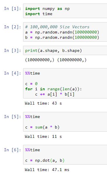
It seems like utilizing NumPy's Dot Product Operation can be ~14x Faster than Explicit For-Loops!
In fact it can be ~1000x Faster when dealing with Larger Arrays as seen in the 100,000,000 sized calculations below
Also, when we utilize Machine Learning Libraries like PyTorch and Tensorflow that utilizes GPU power, 43s can become 4ms
NumPy |
PyTorch |
 |
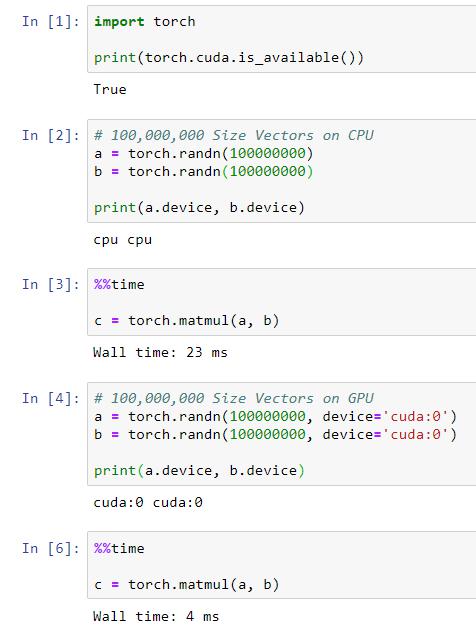 |
The GPU with PyTorch was done on a Desktop Computer with an nVidia GPU (We won't be able to do that with Laptop Integrated Graphics unless you're a hardcore gamer and you have your dedicated graphics properly set up).
Or, we could use Cloud Computing Services).
2 Apples + 1 Banana will Cost $13
3 Apples + 2 Banana will Cost $22
Vectorize the Information as:
$\left[ {\begin{array}{c} 2 & 1 \\ 3 & 2\end{array} } \right] . \left[ {\begin{array}{c} A \\ B\end{array} } \right] = \left[ {\begin{array}{c} 13 \\ 22\end{array} } \right]$
Dot Product would give us:
$\left[ {\begin{array}{c} 2A + 1B \\ 3A + 2B\end{array} } \right] = \left[ {\begin{array}{c} 13 \\ 22\end{array} } \right]$
Think of Rows as Samples, Columns as Variables for Each Item {A, B}
Solving {A, B} is not the Point here, the Representation of Data by Vectorization is the Point.
A = 4
B = 5
Solving with Linear Algebra
units = np.array([[2,1], [3,2]])
cost = np.array([13,22])
np.linalg.inv(units) @ cost
2 Apples + 1 Banana will Cost $12
3 Apples + 2 Banana will Cost $19
New Variable: Ordering Cost of $O/Purchase
O = ?
Vectorize the Information as:
$\left[ {\begin{array}{c} 2 & 1 \\ 3 & 2\end{array} } \right] . \left[ {\begin{array}{c} A \\ B\end{array} } \right] + O = \left[ {\begin{array}{c} 12 \\ 19\end{array} } \right]$
Dot Product would give us:
$\left[ {\begin{array}{c} 2A + 1B \\ 3A + 2B\end{array} } \right] + O = \left[ {\begin{array}{c} 12 \\ 19\end{array} } \right]$
Broadcast O:
$\left[ {\begin{array}{c} 2A + 1B + O\\ 3A + 2B + O\end{array} } \right] = \left[ {\begin{array}{c} 12 \\ 19\end{array} } \right]$
Think of Rows as Samples, Columns as Variables for Each Item {A, B}
Again, Solving {A, B, O} is not the Point here, the Representation of Data by Vectorization is the Point.
A = 3
B = 4
O = 2
Note that we can always re-write as:
$\left[ {\begin{array}{c} 2 & 1\\ 3 & 2\end{array} } \right] . \left[ {\begin{array}{c} A \\ B\end{array} } \right] = \left[ {\begin{array}{c} 12-O \\ 19-O\end{array} } \right]$
or
$\left[ {\begin{array}{c} 2 & 1 & 1\\ 3 & 2 & 1\end{array} } \right] . \left[ {\begin{array}{c} A \\ B\\ O \end{array} } \right] = \left[ {\begin{array}{c} 12 \\ 19\end{array} } \right]$
2 Apples + 1 Banana will Cost $13
3 Apples + 2 Banana will Cost $18
New Variable: Ordering Cost of $2/Purchase
O = 2
Vectorize the Information as:
$\left[ {\begin{array}{c} 2 & 1 \\ 3 & 2\end{array} } \right] . \left[ {\begin{array}{c} A \\ B\end{array} } \right] + 2 = \left[ {\begin{array}{c} 13 \\ 18\end{array} } \right]$
Dot Product would give us:
$\left[ {\begin{array}{c} 2A + 1B \\ 3A + 2B\end{array} } \right] + 2 = \left[ {\begin{array}{c} 13 \\ 18\end{array} } \right]$
Broadcast 2:
$\left[ {\begin{array}{c} 2A + 1B + 2\\ 3A + 2B + 2\end{array} } \right] = \left[ {\begin{array}{c} 13 \\ 18\end{array} } \right]$
Now we shift our focus to Finding the Best Estimate of A and B, to minimize the Error in Predicted Cost
For Instance:
A = 3
B = 4
$Predicted = \left[ {\begin{array}{c} 2 & 1 \\ 3 & 2\end{array} } \right] . \left[ {\begin{array}{c} 3 \\ 4\end{array} } \right] + 2$
$= \left[ {\begin{array}{c} 2\times3 + 1\times4 \\ 3\times3 + 2\times4\end{array} } \right] + 2$
$= \left[ {\begin{array}{c} 6 + 4\\ 9 + 8\end{array} } \right] + 2$
$= \left[ {\begin{array}{c} 10\\ 17\end{array} } \right] + 2$
$= \left[ {\begin{array}{c} 12 \\ 19\end{array} } \right]$
$Error = Prediction - Actual$
$Error = \left[ {\begin{array}{c} 12 \\ 19\end{array} } \right] - \left[ {\begin{array}{c} 13 \\ 18\end{array} } \right]$
$= \left[ {\begin{array}{c} -1 \\ 1\end{array} } \right]$
Are there better answers?
To see how we can minimize Error, we will look into Differentiation in the Part 2.
Demonstration of the Use of Linear Algebra in Machine Learning / Data Analysis
prices = pd.read_csv('./sources/prices.csv', index_col=0)
prices.head()
returns = prices.pct_change().dropna()
returns.head()
returns.describe()
Principal Component Analysis
corr_matrix = returns.corr()
print(corr_matrix)
eigvals, eigvecs = np.linalg.eig(corr_matrix) # Eigen-decomposition of the Correlation Matrix
idx = np.argsort(eigvals)[::-1]
eigvals = eigvals[idx]
eigvecs = eigvecs[:, idx]
var_contri = eigvals / eigvals.sum()
plt.title('Scree Plot', fontsize=16)
plt.plot(var_contri, c='blue')
plt.show();

fig = plt.figure(figsize=(10,4))
plt.title('Principal Components', fontsize=16)
colors = ['blue', 'purple', 'orange']
num = 3
for i in range(3):
    plt.plot(eigvecs[:,i], c=colors[i])
    plt.scatter(returns.columns, eigvecs[:,i], c=colors[i], label='PC{} {:.2f}%'.format(i+1, var_contri[i]*100))
plt.legend()
plt.show();

Monte Carlo Simulations
L = np.linalg.cholesky(returns.cov()) # Cholesky Decomposition of Covariance Matrix
portfolios = np.array([eigvecs[:,i]/eigvecs[:,i].sum() for i in range(len(eigvals))])
n_sims = 10000
z = np.random.randn(n_sims, 252, len(L))
x = z @ L.T + returns.mean().values
sim_rets = ((x+1).prod(axis=1)-1) @ portfolios.T
for i in range(len(portfolios)):
    print(f'Portfolio {i+1}')
    print('Mean Returns: {:.2f}% | Volatility: {:.2f}%'.format(sim_rets[:,i].mean()*100, sim_rets[:,i].std()*100))
plt.title('Returns Distribution') # Returns Distribution of Portfolio 1
plt.hist(sim_rets[:,0], bins=20)
plt.show();

VAR = np.quantile(sim_rets[:,0], 0.05)
print('{:.2f}%'.format(VAR*100)) # Value at Risk % - 5% Chance to Lose More than:
CVAR = sim_rets[:,0][sim_rets[:,0] < VAR].mean()
print('{:.2f}%'.format(CVAR*100)) # Conditional Value at Risk % - 5% to Lose: