![]()
Machine Learning Programming Workshop
1.1 Introduction to Machine Learning
Prepared By: Cheong Shiu Hong (FTFNCE)
What is Machine Learning?
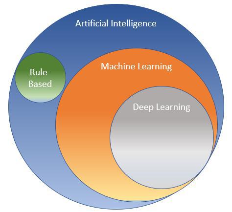
Machine Learning as a Sub-Set of Artificial Intelligence
A Way to Achieve Artificial Intelligence
Deep Learning as a Specialized Form of Machine Learning
Machine Learning and Deep Learning has picked up its pace in the past few years due to:
- Increase in Computational Power
- Increase in Data
Machine Learning is about:
Experience (Data to Learn From)
Task (Output from the Machine)
Performance (How Well it Performs)
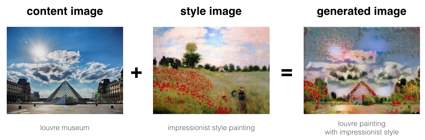
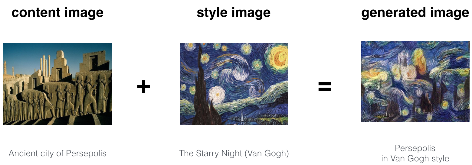
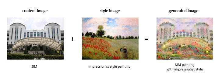
Neural Style Transfer
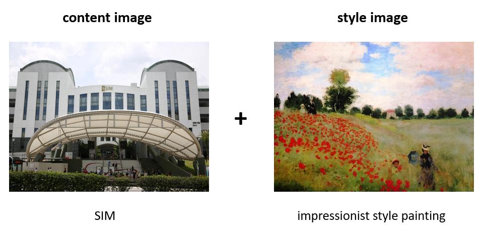
Let's Try Our Own Image:

Reinforcement Learning
Machine Playing Flappy Bird
from IPython.display import YouTubeVideo
YouTubeVideo('aeWmdojEJf0')
Use Cases:
Finance:
Anomaly Detection
Robo-advising
Algorithmic Trading
Machine learning in finance: Why, what & how
JPMorgan's new guide to machine learning in algorithmic trading
Human Resources:
Optimization of Staffing
Talent Management
Resume Screening
Marketing:
Optimization of Message Targeting
Improved Propensity Models and Segmentation
Optimization of Marketing Mix
Supply Chain:
Physical Inspection with Computer Vision
Improved Production Planning and Factory Scheduling
Extension of Lives of Supply Chain Assets
How To Improve Supply Chains With Machine Learning: 10 Proven Ways
10 Ways Machine Learning Is Revolutionizing Supply Chain Management
Analytics:
- You Don't Say
Types of Machine Learning:
Supervised Learning
Unsupervised Learning
Reinforcement Learning
Given a dataset, knowing what the correct outputs are, with the assumption that there is some underlying relationship between the inputs and outputs.
We try to predict Y, given some data X where:
X: Inputs (Features)
Y: Output(s) (Labels)
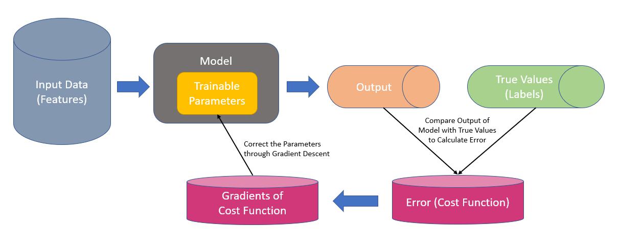
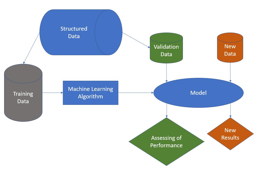
We train the model not with all the data we have. It would make make more sense to reserve some of the data to be used to evaluate the model's performance on unseen data.
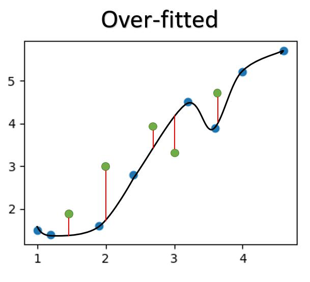
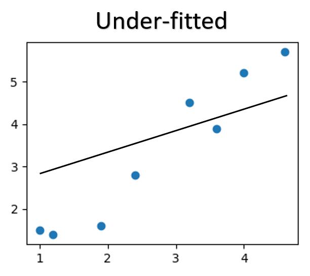
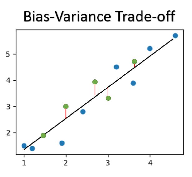
Bias-Variance Trade-off
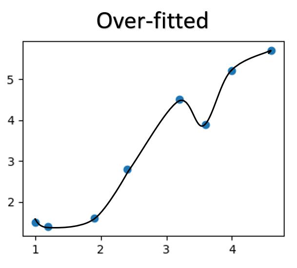
When we train the model, the algorithm's goal is to train the model to best fit the data provided for training. However, there will be a tendency for the model to be OVERFITTED to the training data, where the model 'Memorizes' the data and perform extremely well on the training set, but preforms poorly on new unseen data.
 |
 |
On the other hand, we can not accept an underfitted model that does not even perform reasonably well.
 |
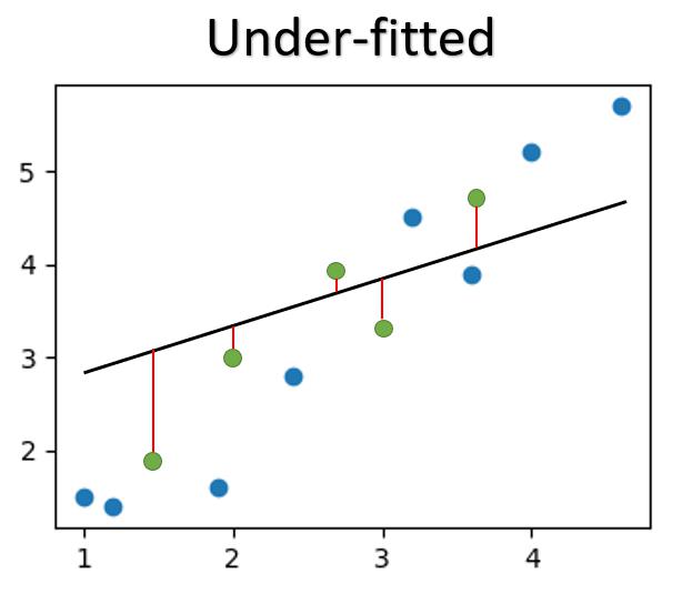 |
Therefore, this is known as the Bias-Variance Trade-off where we want to minimize BIAS (the ability of the model to provide correct predictions based on the training data, without sacrificing VARIANCE (how well the model performs on new unseen data).
When we overtrain the model, the model can be OVERFITTED, performing well on the training data, but poorly on new unseen data.
When we undetraing the model, the model can be UNDERFITTED, showing average or poor performance on both the training data and validation data.
Ideally, we would want a model that is able to generalise capture the relationship reasonably well, while also minimizing error for new unseen data without overfitting to the training data.
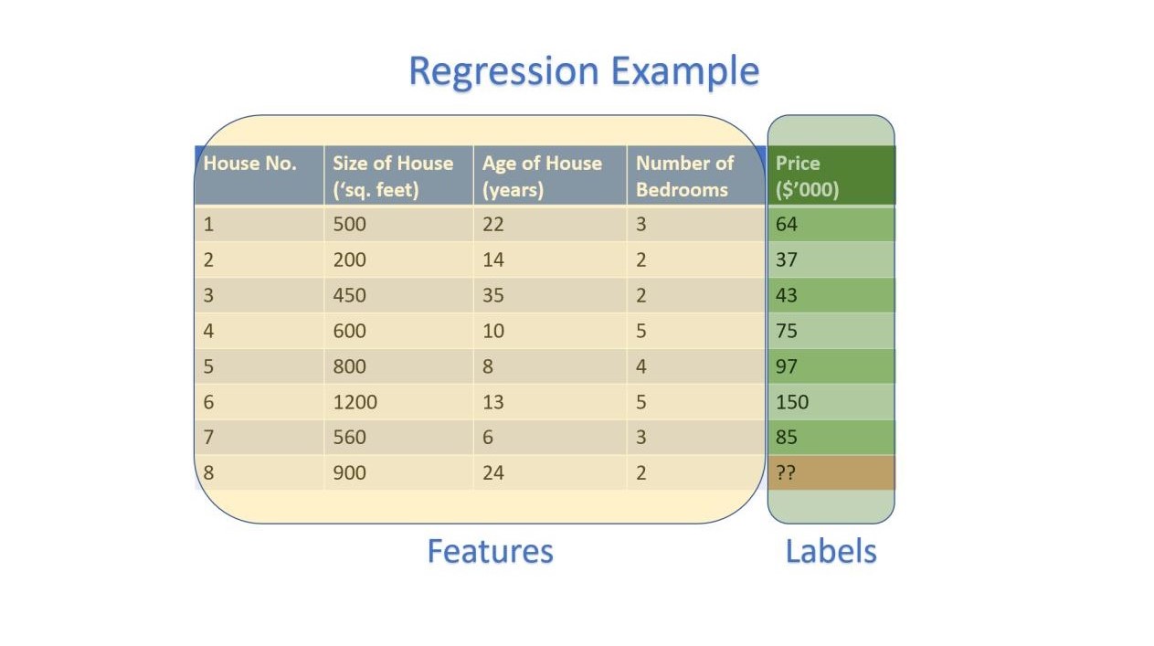
Regression
E.g. Predicting Prices of Houses given the Size and Age of these Houses
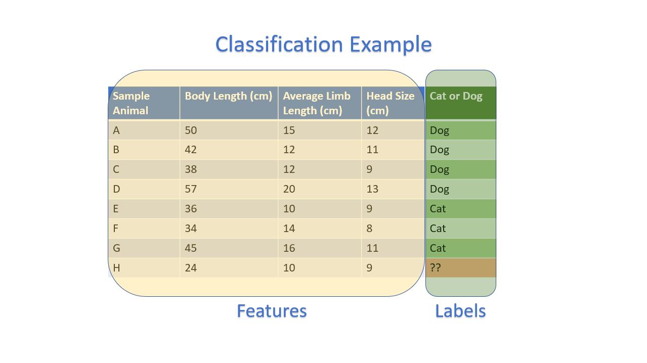
Classification
E.g. Predicting if an Animal is a Cat or a Dog
By knowing what Inputs we have, and what Outputs we want from the Model, we can choose an intuitive and relevant model.
Choose a Model:
For a start, let's use a model that should be familiar with all of us, The Linear Regression Model
$\hat{y} = w.x + b$
Where [$w$] is the Gradient (Slope) of the Line, and [$b$] is the Y-Intercept
$m$ = number of samples
$n$ = number of features
Therefore, the number of parameters to be optimized in the model are:
$n + 1$ (1 parameter for each feature, + 1 parameter for Y-Intercept)
Goal: Fit the Best Fit Line (Least Error) --> (Least Sums of Squared Error)
Since Error can be both positive or negative, we use Squared Error as our metric.
Error is measured by: $\hat{y} - y$
Squared Error is measured by: $(\hat{y} - y)^2$
Sums of Squared Error is measured by: $\sum\limits_{i=1}^{m}(\hat{y}_{i} - y_{i})^2$
In Simple Linear Regression, we can easily solve for the Optimal [$w$] and [$b$] by using a familiar formula (Hint: BUS105):
$w = \frac{cov(x, y)}{var(x)} = \frac{\sum\limits_{i=1}^{m}(x_i - \bar{x})(y_i - \bar{y})}{\sum\limits_{i=1}^{m}(x_i - \bar{x})^2} = \frac{\sum\limits_{i=1}^{m}(x_i - \bar{x})(y_i - \bar{y})}{\sum\limits_{i=1}^{m}(x_i - \bar{x})(x_i - \bar{x})}$
$b = \bar{y} - w.\bar{x}$
However, when the number of features (dimensions) increase, the problem becomes more and more complex to solve directly.
Consider the below images on Regressions with 2 Features, $X_1$ and $X_2$:
Regression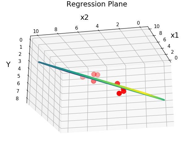
|
Classification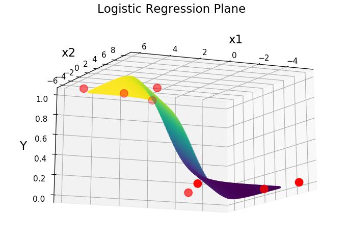
|
|---|
A common way to solve [$w_1, w_2$, ..., $w_n$] and [$b$] would be to use normal equations, through differentiation of the Error Function, to find the gradient of the Error Function with respect to each parameter {$w_1, w_2$, ..., $w_n, b$}, and finding the corresponding parameters that allows the gradients to be 0 (Minimum Error).
However, as the problem becomes more and more complex, solving by normal equations becomes less and less efficient.
For a scalable way to find optimal values of [$w_1, w_2$, ..., $w_n$] and [$b$], we will introduce Gradient Descent later on.
With little or no idea of what our outputs should look like, there is no evaluation metric for any predictions by the model. However, Machine Learning still enables us to find patterns and structure from datasets, by clustering similar samples together.
Unsupervised Learning is more exploratory since there is no clear objective, without any true answers for the model to produce.
X: Inputs (Features)
Machine will find simlarity and patterns in data without 'Predictions'
Two Main Techniques:
- Principal Component Analysis
- Clustering
Principal Component Analysis
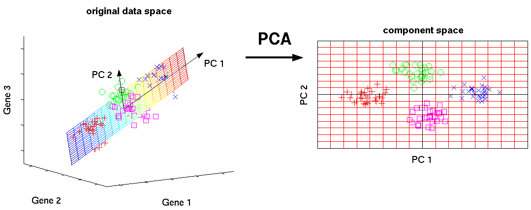
The process of deriving Principal Components is to better understand the data, as well as visualize the data through dimensionality reduction.
With Principal Component Analysis, we can identify a lower-dimension representation of the dataset through basis transformation, that contains the most variations in the new basis, while lower variations that are not as interesting are ignored. (Components with higher variations are considered more interesting)
Clustering Methods
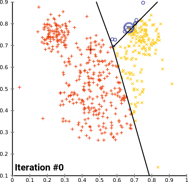
Clustering refers to finding subgroups within a dataset, without the data being explicitly labelled as a certain 'category'.
Example: In dealing with Customer Data, we want to group customers together that have similar habits, and through clustering, we can identify groups of customers that are likely to behave or react similarly.
In Clustering, [$K$] refers to the number of subgroups or number of clusters. ($K=2$ means 2 clusters, $K = 5$ means 5 clusters)
- K Means Clustering
- Hierachical Clustering

In Reinforcement Learning, the goal is to train an agent to perform a certain task.
In the examples above, a machine can learn to play Flappy Bird through Reinforcement Learning
The Machine will have no clue of what Flappy Bird is, or what the purpose of the game is.
Benefits of Reinforcement Learning include:
- Better than Human-Level Performance (a.k.a Bayes Error Rate)
- No need for complicated labels
Bayes Error Rate (Maximum Human Performance for a Task): If we train a machine to perform a task with Supervised Learning based on our Human-Created Labels, the Machine can only perform at our Human-Level AT BEST.
Example: Open.AI Artificial Intelligence Beating Top Teams in DotA 2. The AI did not learn excessively from humans, but instead starts off by randomly doing random things in the game, to learn which actions or set of actions provided rewards, vs penalties; potentially exploiting the game to it's advantage. This way, Machines are able to outperform Humans in certain tasks.
Turns out, Reinforcement Learning is effective not only in playing games, but also in many other areas, as long as the rewards are well structured.
Machine Learning is a way to find complex relationships between variables and before jumping into Machine Learning, the Problem and Task has to be defined.
Data Acquisition
Data can be acquired intentionally for a specific purpose, or non-intentionally.
Data Exploration
Exploring the relationships of the data through Visualization and Analysis
Are there correlations in the data?
Define the Task
What is the task that Machine Learning can be applied to?
Is it a Classification task, Regression Task, or Action-Based Task?
Are there intuitive relationships between the independent and dependent variables?
Data Preparation
After understanding which variables are of interest, these data will need to be processed and prepared in order to be applicable to the task as inputs to a model.
Choosing a Model
What relationships do the variables have? Linear? Non-Linear?
What kind of Model would be suitable to replicate the believed underlying relationship of the variables?
Training the Model
Feed the Data into the Algorithm to Train the Model.
Evaluation and Refinement
Parameter Tuning - Improving the Model by tuning Hyperparameters of the Algorithm to train the Model.
Exploring other Models - Can other Models that might not seem as the obvious solution perform better?
Deployment
Using the Model to generate predictions for actual use.