![]()
Machine Learning Programming Workshop
3.3 Tensorflow/Keras (Computer Vision)
Prepared By: Cheong Shiu Hong (FTFNCE)
In [1]:
import numpy as np
import pandas as pd
import matplotlib.pyplot as plt
import time
In [2]:
import tensorflow as tf
import tensorflow.keras as K
Version of Tensorflow and Keras
In [3]:
tf.__version__
Out[3]:
In [4]:
K.__version__ # tf means Tensorflow Backend
Out[4]:
Load Dataset
In [5]:
data = K.datasets.fashion_mnist
In [6]:
(train_images, train_labels), (val_images, val_labels) = data.load_data()
How do computer see images?
Each image is a 28x28 Array carrying values of pixel intensity
In [7]:
train_images[0].shape
Out[7]:
In [8]:
img_size = train_images[0].shape[0]
print(img_size)
In this demonstration, images are of low resolution (28x28) and are Black & White
What would the array look like for RGB images?
Normally, we will have to pre-process the images to standardize the resolution and shape of the image.
Numpy - Tranpose, Reshape, Resize
In [9]:
train_images.shape, train_labels.shape
Out[9]:
In [10]:
val_images.shape, val_labels.shape
Out[10]:
In [11]:
class_names = [
    'T-Shirt/Top',
    'Trousers',
    'Pullover',
    'Dress',
    'Coat',
    'Sandal',
    'Shirt',
    'Sneaker',
    'Bag',
    'Ankle Boot'
]

num_classes = len(class_names)
In [12]:
horiz = 5; vert = 3; area = vert*horiz;
fig = plt.figure(figsize=(12,8))
for i in range(area):
    ax = plt.subplot(vert,horiz,i+1)
    ax.set_title(class_names[train_labels[i]])
    ax.imshow(train_images[i])#, cmap=plt.cm.binary)n

Rescale Arrays (Image arrays have large integer values)
Pixel values need not be of any distribution, but its range is between 0 and 255.
In [13]:
train_images = train_images / 255.0
val_images = val_images / 255.0
Reshape Images (Flatten)
In [14]:
reshaped_train = train_images[:2500].reshape(2500, img_size*img_size)
reshaped_val = val_images[:2500].reshape(2500, img_size*img_size)
In [15]:
reshaped_train.shape, reshaped_val.shape
Out[15]:
Logistic Regression
In [16]:
from sklearn.linear_model import LogisticRegression
In [17]:
log_reg = LogisticRegression()
In [18]:
log_reg.fit(reshaped_train, train_labels[:2500])
Out[18]:
In [19]:
log_reg.score(reshaped_val, val_labels[:2500])
Out[19]:
Let's Build a Neural Network with Keras
In [20]:
model = K.Sequential([
    K.layers.Flatten(input_shape=(img_size, img_size)), # Flattens 28 x 28 Image into 784
    K.layers.Dense(32, activation='relu'),
    K.layers.Dense(16, activation='relu'),
    K.layers.Dense(num_classes, activation='softmax')
])
In [21]:
model.compile(optimizer='adam', loss='sparse_categorical_crossentropy', metrics=['accuracy'])
In [22]:
model.fit(train_images, train_labels, epochs=5, batch_size=32)
Out[22]:
In [23]:
model.evaluate(val_images, val_labels) # ADAM
Out[23]:
In [24]:
model.predict([[val_images[0]]])
Out[24]:
In [25]:
fig = plt.figure(figsize=(15,7))
for i in range(10):
    ax = plt.subplot(2,5,i+1)
    ax.imshow(val_images[i], cmap=plt.cm.binary)
    ax.set_title('Actual: {}'.format(class_names[val_labels[i]]))
    ax.set_xlabel('Predicted: {}'.format(class_names[np.argmax(model.predict([[val_images[i]]]))]))

Keras Conv2D Layer takes in (B, Sv, Sh, C) where C is the the number of channels (3 for RGB, 1 for Black & White)
PyTorch's Convolutional Layer in contrast, takes in (B, C, Sv, Sh)
In [26]:
conv_train_images = train_images.reshape(train_images.shape[0], img_size, img_size, 1)
conv_val_images = val_images.reshape(val_images.shape[0], img_size, img_size, 1)
In [27]:
conv_train_images.shape, conv_val_images.shape
Out[27]:
In [28]:
conv_model = K.Sequential([
    K.layers.Conv2D(8, (3,3), padding='same', activation='relu'),
    K.layers.MaxPooling2D(pool_size=(2,2)),
    K.layers.Conv2D(8, (3,3), padding='same', activation='relu'),
    K.layers.MaxPooling2D(pool_size=(2,2)),
    K.layers.Flatten(),
    K.layers.Dense(16, activation='relu'),
    K.layers.Dense(8, activation='relu'),
    K.layers.Dense(num_classes, activation='softmax')
])
In [29]:
conv_model.compile(optimizer='adam', loss='sparse_categorical_crossentropy', metrics=['accuracy'])
In [30]:
conv_model.fit(conv_train_images, train_labels, epochs=5)
Out[30]:
In [31]:
conv_model.evaluate(conv_val_images, val_labels)
Out[31]:
In [32]:
fig = plt.figure(figsize=(15,7))
for i in range(10):
    ax = plt.subplot(2,5,i+1)
    ax.imshow(val_images[i], cmap=plt.cm.binary)
    ax.set_title('Actual: {}'.format(class_names[val_labels[i]]))
    ax.set_xlabel('Predicted: {}'.format(class_names[np.argmax(conv_model.predict([[conv_val_images[i]]]))]))

Compare the Models</h1>
Artificial Neural Network
In [33]:
model.summary()
Convolutional Neural Network
In [34]:
conv_model.summary()
Convolutional Layers have less Trainable-Parameters and are comparatively less expensive than Dense/Recurrent Layers
Especially with GPU, when Convolutional Compuations are Parallelized with large Bandwidths, Convolutional Neural Networks are very effective and efficient
Can't calculate later layers before earlier layers are done, thus not too much difference between CPU and GPU
But intra-layer, each node can be calculated simultaneously, thus GPUs show advantage in parallelized computations with larger bandwidths, especially for Convolutional Layers where the same set of (3x3) Parameters are used to multiply on each set of (3x3) Pixels.
In [35]:
from tensorflow.keras.datasets import cifar10
In [36]:
data = cifar10.load_data() # ~170 Megabytes of 60,000 Images in 32 x 32 x 3
In [37]:
(X_train, Y_train), (X_val, Y_val) = data
In [38]:
X_train.shape, Y_train.shape, X_val.shape, Y_val.shape
Out[38]:
In [39]:
img_size = X_train.shape[1]
num_channels = X_train.shape[3]
In [40]:
class_names = [
    'airplane',
    'automobile',
    'bird',
    'cat',
    'deer',
    'dog',
    'frog',
    'horse',
    'ship',
    'truck'
]

num_classes = len(class_names)
In [41]:
fig = plt.figure(figsize=(15,8))
for i, image in enumerate(X_train[:10]):
    ax = plt.subplot(2, 5, i+1)
    ax.imshow(image)
    ax.set_title('Actual: {}'.format(class_names[Y_train[i][0]]))

Scale Pixel Values to 0-1
In [42]:
X_train = X_train / 255.
X_val = X_val / 255.
In [43]:
X_train.shape
Out[43]:
Build Model
In [44]:
conv_model = K.Sequential([
    K.layers.Conv2D(32, (3,3), padding='same', activation='relu', input_shape=(32,32,3,)),
    K.layers.MaxPooling2D(pool_size=(2,2)),
    K.layers.Conv2D(16, (3,3), padding='same', activation='relu'),
    K.layers.MaxPooling2D(pool_size=(2,2)),
    K.layers.Conv2D(8, (3,3), padding='same', activation='relu'),
    K.layers.MaxPooling2D(pool_size=(2,2)),
    K.layers.Flatten(),
    K.layers.Dense(32, activation='relu'),
    K.layers.Dense(num_classes, activation='softmax')
])
In [45]:
conv_model.compile(optimizer='adam', loss='sparse_categorical_crossentropy', metrics=['accuracy'])
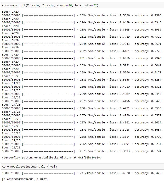
Train Model
In [46]:
conv_model.fit(X_train, Y_train, epochs=2, batch_size=32)
Out[46]:
The good thing about working in Jupyter Notebook is that you can continue training the model in the next cell without saving the model
In [47]:
# Epoch 3
conv_model.fit(X_train, Y_train, epochs=1, batch_size=32, verbose=0) # You can play around with the different arguments
# Verbose 0 means Silent (Nothing printed out)
Out[47]:
In [48]:
# Epoch 4
conv_model.fit(X_train, Y_train, epochs=1, batch_size=32, verbose=2) # You can play around with the different arguments
# Verbose 2 means no Progress Bar (Default is Verbose 1, with Progress Bar)
Out[48]:
In [49]:
# Epoch 5
conv_model.fit(X_train, Y_train, epochs=1, batch_size=32, ) # You can play around with the different arguments
# Verbose 2 means no Progress Bar (Default is Verbose 1, with Progress Bar)
Out[49]:
Evaluate Performance of Model
In [50]:
conv_model.evaluate(X_val, Y_val)
Out[50]:
In [51]:
fig = plt.figure(figsize=(15,7))
for i in range(10):
    ax = plt.subplot(2,5,i+1)
    ax.imshow(X_val[i], cmap=plt.cm.binary)
    ax.set_title('Actual: {}'.format(class_names[Y_val[i][0]]))
    ax.set_xlabel('Predicted: {}'.format(class_names[np.argmax(conv_model.predict([[X_val[i]]]))]))

Saving / Loading the Model
Saving the Model
In [52]:
conv_model.save('conv_model.h5')
Deleting the Model
In [53]:
del conv_model
In [54]:
try: print(conv_model)
except: print("NameError: name 'conv_model' is not defined")
Loading the Model from saved file
In [55]:
conv_model = K.models.load_model('conv_model.h5')
In [56]:
conv_model.evaluate(X_val, Y_val)
Out[56]:
Testing the Model with New Images
In [57]:
import os
from PIL import Image
In [58]:
root = './sources/test_images/'

full_images = []
filenames = [name for name in os.listdir(root)]

for filename in filenames:
    img = Image.open(root+filename)
    img.load()
    full_images.append(np.asarray(img, dtype='int32'))
In [59]:
fig = plt.figure(figsize=(15,8))
for i, image in enumerate(full_images):
    ax = plt.subplot(2, 5, i+1)
    ax.imshow(image)
    ax.set_title('Filename: {}'.format(filenames[i]))

Reload images as 32 x 32 x 3 Arrays
In [60]:
images = []
filenames = [name for name in os.listdir(root)]
root = './sources/test_images/'
for filename in filenames:
    img = Image.open(root+filename)
    img.load()
    img = img.resize(size=(img_size, img_size))
    images.append(np.asarray(img, dtype='int32'))
images = np.array(images)
In [61]:
fig = plt.figure(figsize=(15,8))
for i, image in enumerate(images):
    ax = plt.subplot(2, 5, i+1)
    ax.imshow(image)
    ax.set_title('Filename: {}'.format(filenames[i]))

Predictions
In [62]:
preds = np.argmax(conv_model.predict([images]), 1)
In [63]:
print(preds)
In [64]:
fig = plt.figure(figsize=(15,8))
for i, image in enumerate(full_images):
    ax = plt.subplot(2, 5, i+1)
    ax.imshow(image)
    ax.set_title('Filename: {}'.format(filenames[i]))
    ax.set_xlabel('Predicted: {}'.format(class_names[preds[i]]))

How to further improve?
Dropout Reglarization and Batch Normalization
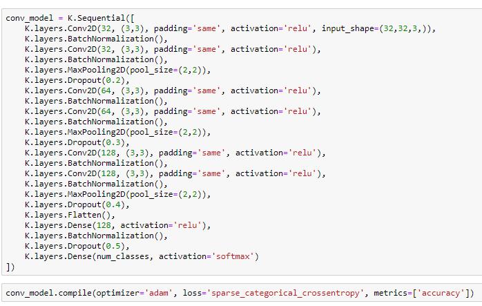
Data Augmentation
Color Augmentation
Cropping
Rotating
Flipping
You can even load models pre-trained on large datasets and retrain only the last few layers
Previous:
Next: