![]()
Machine Learning Programming Workshop
3.2 Introduction to Neural Networks
Prepared By: Cheong Shiu Hong (FTFNCE)
import numpy as np
import pandas as pd
import matplotlib.pyplot as plt
import sklearn as sk
from sklearn import datasets
import time
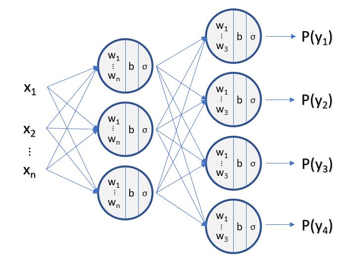
Knowing what Multi-Class Logistic Regression is, we can simply Add Layers for it to be considered a Neural Network:
2-Layer Neural Network (1 Hidden Layer): $(L=2)$
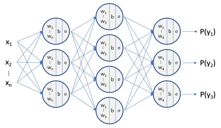
3-Layer Neural Network (2 Hidden Layers): $(L=3)$
Notation Alert:
$\large A_{<l>}$ indicates that this is $\large A$ (Activated Output) in the $\large l^{th}$ Layer
E.g. $Z_{<2>}$ indicates this is the Pre-Activation Function Output in the Second Layer.
In the First Hidden Layer: $(l=1)$
$Z_{<1>} = W_{<1>}^{T} X + B_{<1>}$
$A_{<1>} = \sigma(Z_{<1>})$, where $\sigma$ is the Chosen Activation Function
In the Second Hidden Layer: $(l=2)$
$Z_{<2>} = W_{<2>}^{T} A_{<1>} + B_{<2>}$
$A_{<2>} = \sigma(Z_{<2>})$, where $\sigma$ is the Chosen Activation Function
In the Final (Output) Layer: $(l=L=3)$
$Z_{<3>} = W_{<3>}^{T} A_{<2>} + B_{<3>}$
$\hat{Y} = \sigma(Z_{<3>})$, where $\sigma$ is the Softmax Activation Function
When do we use Dot-Product and Element-Wise Multiplication when calculating Gradients?
In the Final (Output) Layer: $(l=L=3)$
Similar to Multi-Class Logistic Regression, the Gradients of $\hat{Y}$ and $Z_{<3>}$ are:
$\frac{dCost}{d\hat{Y}} = \frac{\hat{Y} - Y}{\hat{Y} (1 - \hat{Y})}$
$\frac{d\hat{Y}}{dZ_{<3>}} = \hat{Y}(1 - \hat{Y})$
Therefore:
$\frac{dCost}{dZ_{<3>}} = \frac{dCost}{d\hat{Y}} \times \frac{d\hat{Y}}{dZ_{<3>}}$
$= \frac{\hat{Y} - Y}{\hat{Y} (1 - \hat{Y})} \times \hat{Y}(1 - \hat{Y})$
$= \hat{Y} - Y$
Parameters to Update:
$W_{<3>}, B_{<3>}, W_{<2>}, B_{<2>}, W_{<1>}, B_{<1>}$
$\frac{dCost}{dW_{<3>}} = \frac{dCost}{d\hat{Y}} \times
\frac{d\hat{Y}}{dZ_{<3>}} \times
\frac{dZ_{<3>}}{dW_{<3>}}$
$\frac{dCost}{dB_{<3>}} = \frac{dCost}{d\hat{Y}} \times
\frac{d\hat{Y}}{dZ_{<3>}} \times
\frac{dZ_{<3>}}{dB_{<3>}}$
$\frac{dCost}{dW_{<2>}} = \frac{dCost}{d\hat{Y}} \times
\frac{d\hat{Y}}{dZ_{<3>}} \times
\frac{dZ_{<3>}}{dA_{<2>}} \times
\frac{dA_{<2>}}{dZ_{<2>}} \times
\frac{dZ_{<2>}}{dW_{<2>}}$
$\frac{dCost}{dB_{<2>}} = \frac{dCost}{d\hat{Y}} \times
\frac{d\hat{Y}}{dZ_{<3>}} \times
\frac{dZ_{<3>}}{dA_{<2>}} \times
\frac{dA_{<2>}}{dZ_{<2>}} \times
\frac{dZ_{<2>}}{dB_{<2>}}$
$\frac{dCost}{dW_{<1>}} = \frac{dCost}{d\hat{Y}} \times
\frac{d\hat{Y}}{dZ_{<3>}} \times
\frac{dZ_{<3>}}{dA_{<2>}} \times
\frac{dA_{<2>}}{dZ_{<2>}} \times
\frac{dZ_{<2>}}{dA_{<1>}} \times
\frac{dA_{<1>}}{dZ_{<1>}} \times
\frac{dZ_{<1>}}{dW_{<1>}}$
$\frac{dCost}{dB_{<1>}} = \frac{dCost}{d\hat{Y}} \times
\frac{d\hat{Y}}{dZ_{<3>}} \times
\frac{dZ_{<3>}}{dA_{<2>}} \times
\frac{dA_{<2>}}{dZ_{<2>}} \times
\frac{dZ_{<2>}}{dA_{<1>}} \times
\frac{dA_{<1>}}{dZ_{<1>}} \times
\frac{dZ_{<1>}}{dB_{<1>}}$
Similar to Multi-Class Logistic Regression, the Gradients of $\hat{Y}$ and $Z_{<3>}$ are:
$\frac{dCost}{d\hat{Y}} = \frac{\hat{Y} - Y}{\hat{Y} (1 - \hat{Y})}$
$\frac{d\hat{Y}}{dZ_{<3>}} = \hat{Y}(1 - \hat{Y})$
Therefore:
$\frac{dCost}{dZ_{<3>}} = \frac{dCost}{d\hat{Y}} \times \frac{d\hat{Y}}{dZ_{<3>}}$
$= \frac{\hat{Y} - Y}{\hat{Y} (1 - \hat{Y})} \times \hat{Y}(1 - \hat{Y})$
$= \hat{Y} - Y$
The Gradients of the Weights and Biases are:
$\frac{dZ_{<3>}}{dW_{<3>}} = A_{<2>}$
$\frac{dZ_{<3>}}{dB_{<3>}} = 1$
And:
$\frac{dCost}{dW_{<3>}} = \frac{dCost}{dZ_{<3>}} \times \frac{dZ_{<3>}}{dW_{<3>}}$
$\frac{dCost}{dB_{<3>}} = \frac{dCost}{dZ_{<3>}} \times \frac{dZ_{<3>}}{dB_{<3>}}$
Therefore:
$\frac{dCost}{dW_{<3>}} = (\hat{Y} - Y) \times A_{<2>}^{T}$ (n_C, m) x (m, n_H2)
$\frac{dCost}{dW_{<3>}} = (\hat{Y} - Y) A_{<2>}^{T}$ (n_C, n_H2)
$\frac{dCost}{dB_{<3>}} = (\hat{Y} - Y) \times 1$
$\frac{dCost}{dB_{<3>}} = \hat{Y} - Y$
In the Second Hidden Layer: $(l=2)$
The Gradients of $A_{<2>}$ and $Z_{<2>}$ are:
$\frac{dCost}{dA_{<2>}} = \frac{dCost}{d\hat{Y}} \times \frac{d\hat{Y}}{dZ_{<3>}} \times \frac{dZ_{<3>}}{dA_{<2>}}$
$\frac{dCost}{dA_{<2>}} = \frac{dCost}{dZ_{<3>}} \times \frac{dZ_{<3>}}{dA_{<2>}}$
$\frac{dCost}{dA_{<2>}} = (\hat{Y} - Y)^{T} \times W_{<3>}$
$\frac{dCost}{dA_{<2>}} = (\hat{Y} - Y)^{T} W_{<3>}$
$\frac{dA_{<2>}}{dZ_{<2>}} = A_{<2>}(1 - A_{<2>})$
Therefore:
$\frac{dCost}{dZ_{<2>}} = \frac{dCost}{dA_{<2>}} \times \frac{dA_{<2>}}{dZ_{<2>}}$
$= (\hat{Y} - Y)^{T} W_{<3>} \times A_{<2>}(1 - A_{<2>})$ (Element-Wise)
The Gradients of the Weights and Biases are:
$\frac{dZ_{<2>}}{dW_{<2>}} = A_{<1>}$
$\frac{dZ_{<2>}}{dB_{<2>}} = 1$
And:
$\frac{dCost}{dW_{<2>}} = \frac{dCost}{dZ_{<2>}} \times \frac{dZ_{<2>}}{dW_{<2>}}$
$\frac{dCost}{dB_{<2>}} = \frac{dCost}{dZ_{<2>}} \times \frac{dZ_{<2>}}{dB_{<2>}}$
Therefore:
$\frac{dCost}{dW_{<2>}} = [(\hat{Y} - Y)^{T} W_{<3>} \times A_{<2>}(1 - A_{<2>})] \times A_{<1>}^{T}$ (n_H2, m) x (m, n_H1)
$\frac{dCost}{dW_{<2>}} = [(\hat{Y} - Y)^{T} W_{<3>} \times A_{<2>}(1 - A_{<2>})] A_{<1>}^{T}$ (n_H2, n_H1)
$\frac{dCost}{dB_{<2>}} = [(\hat{Y} - Y)^{T} W_{<3>} \times A_{<2>}(1 - A_{<2>})] \times 1$
$\frac{dCost}{dB_{<2>}} = (\hat{Y} - Y)^{T} W_{<3>} \times A_{<2>}(1 - A_{<2>})$
In the First Hidden Layer: $(l=1)$
**Assume Sigmoid as Activation Function
The Gradients of $A_{<1>}$ and $Z_{<1>}$ are:
$\frac{dCost}{dA_{<1>}} = \frac{dCost}{d\hat{Y}} \times \frac{d\hat{Y}}{dZ_{<3>}} \times \frac{dZ_{<3>}}{dA_{<2>}} \times \frac{dA_{<2>}}{dZ_{<2>}} \times \frac{dZ_{<2>}}{dA_{<1>}}$
$\frac{dCost}{dA_{<1>}} = \frac{dCost}{dZ_{<2>}} \times \frac{dZ_{<2>}}{dA_{<1>}}$
$\frac{dCost}{dA_{<1>}} = [(\hat{Y} - Y)^{T} W_{<3>} \times A_{<2>}(1 - A_{<2>})]^{T} \times W_{<2>}$
$\frac{dCost}{dA_{<1>}} = [(\hat{Y} - Y)^{T} W_{<3>} \times A_{<2>}(1 - A_{<2>})]^{T} W_{<2>}$
$\frac{dA_{<1>}}{dZ_{<1>}} = A_{<1>}(1 - A_{<1>})$
Therefore:
$\frac{dCost}{dZ_{<1>}} = \frac{dCost}{dA_{<1>}} \times \frac{dA_{<1>}}{dZ_{<1>}}$
$= [(\hat{Y} - Y)^{T} W_{<3>} \times A_{<2>}(1 - A_{<2>})]^{T} W_{<2>} \times A_{<1>}(1 - A_{<1>})$ (Element-Wise)
The Gradients of the Weights and Biases are:
$\frac{dZ_{<1>}}{dW_{<1>}} = X$
$\frac{dZ_{<1>}}{dB_{<1>}} = 1$
And:
$\frac{dCost}{dW_{<1>}} = \frac{dCost}{dZ_{<1>}} \times \frac{dZ_{<1>}}{dW_{<1>}}$
$\frac{dCost}{dB_{<1>}} = \frac{dCost}{dZ_{<1>}} \times \frac{dZ_{<1>}}{dB_{<1>}}$
Therefore:
$\frac{dCost}{dW_{<1>}} = [[(\hat{Y} - Y)^{T} W_{<3>} \times A_{<2>}(1 - A_{<2>})]^{T} W_{<2>} \times A_{<1>}(1 - A_{<1>})] \times X^{T}$ (n_H1, m) x (m, n_In)
$\frac{dCost}{dW_{<1>}} = [[(\hat{Y} - Y)^{T} W_{<3>} \times A_{<2>}(1 - A_{<2>})]^{T} W_{<2>} \times A_{<1>}(1 - A_{<1>})] X^{T}$ (n_H1, n_In)
$\frac{dCost}{dB_{<1>}} = [[(\hat{Y} - Y)^{T} W_{<3>} \times A_{<2>}(1 - A_{<2>})]^{T} W_{<2>} \times A_{<1>}(1 - A_{<1>})] \times 1$
$\frac{dCost}{dB_{<1>}} = [[(\hat{Y} - Y)^{T} W_{<3>} \times A_{<2>}(1 - A_{<2>})]^{T} W_{<2>} \times A_{<1>}(1 - A_{<1>})]$
Note that:
$\large \frac{dCost}{dB_{<l>}} = dZ_{<l>}$
Also, we do not expand out the $A$s and $\hat{Y}$ as we will cache these values from the Forward Pass.
Backpropagation in Neural Networks
We notice that the Backpropagation of Gradients in a Neural Network works very similarly to that of Linear/Logistic Regressions, except that we have multiple layers and we are stacking the Chain Rule Continuously.
Once Gradients have been passed back through Backpropagation, we can update all the Model Parameters at once with Gradient Descent.
Vanishing & Exploding Gradients
As gradients are continuously multiplied in the backward pass due to the Chain Rule, Neural Networks can suffer from Vanishing/Exploding Gradients as the Network gets Extremely Deep.
Sigmoid

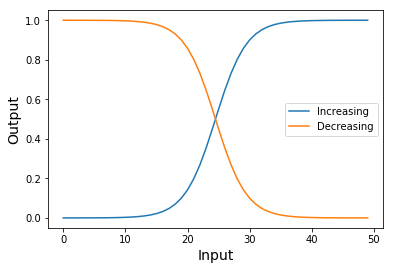
Softmax
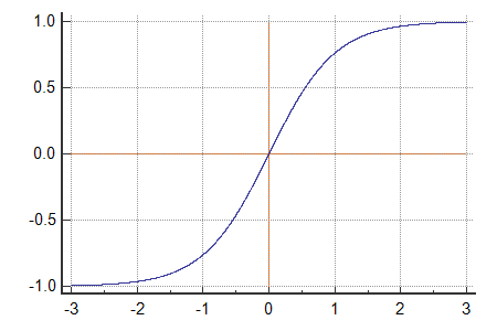
Tanh (Hyperbolic Tangent)
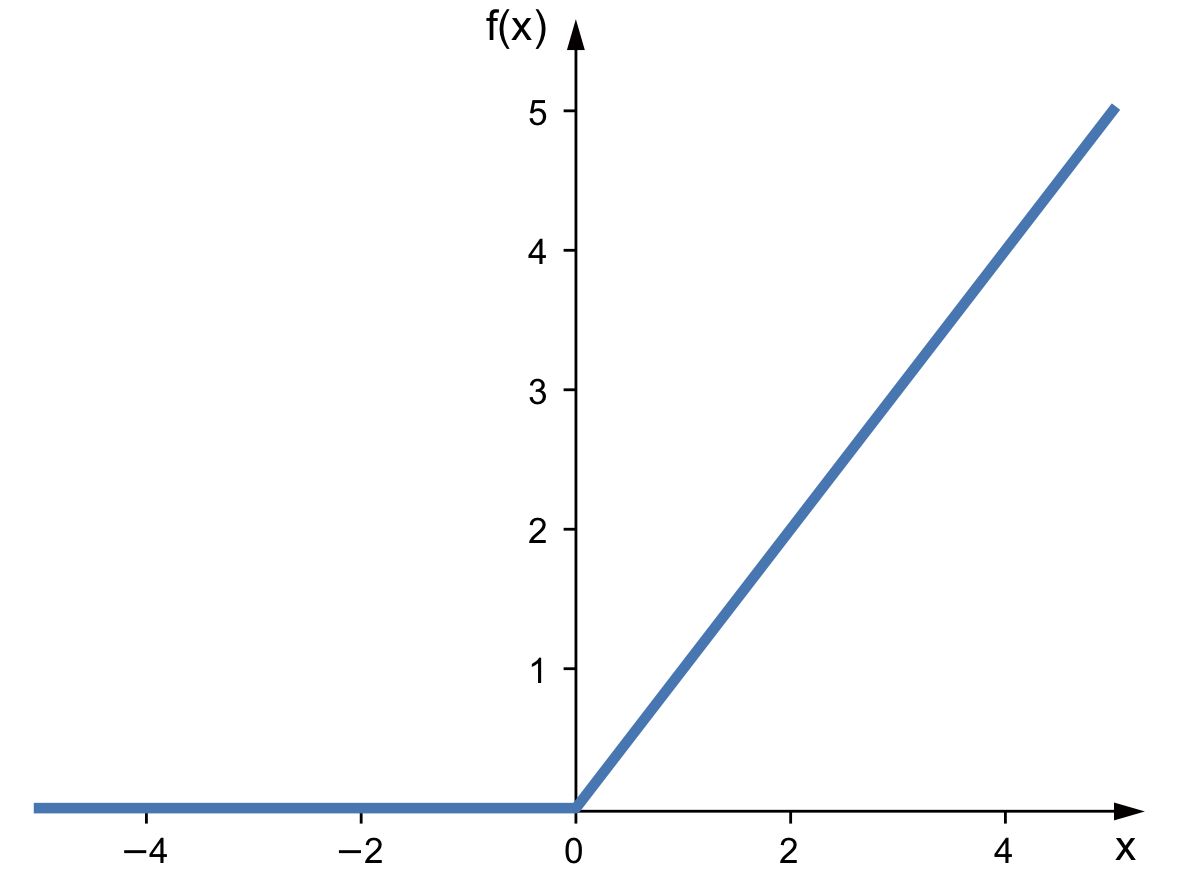
ReLU (Rectified Linear Unit)
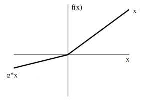
Leaky ReLU (Leaky Rectified Linear Unit)
Iris Dataset Example
iris = datasets.load_iris()
iris.keys()
Define Num Features (n_F) and Num Classes(n_C)
n_F = len(iris['feature_names'])
n_C = len(iris['target_names'])
Shape of X and Y
iris['data'].shape, iris['target'].shape
Visualize Dataset in DataFrame
pd.DataFrame(iris['data'], columns=iris['feature_names']).head()
iris.target_names
X = iris['data'].T
Y_class = iris['target']
X.shape, Y_class.shape
One-Hot Encode Labels
def one_hot(array, num_classes):
    new_array = np.zeros((len(array), num_classes))
    for i, val in enumerate(array):
        new_array[i, val] = 1
    return new_array
Y = one_hot(Y_class, n_C).T
Y.shape
Shuffle Data
indices = np.arange(iris['target'].shape[0])
np.random.shuffle(indices)
X = X[:,indices]
Y = Y[:,indices]
Y_class = Y_class[indices]
Train Test Split
split_ratio = 0.2
split = int(Y.shape[1] * split_ratio)

X_train = X[:, split:]
X_val = X[:, :split]
Y_train = Y[:, split:]
Y_val = Y[:, :split]
Y_class_train = Y_class[split:]
Y_class_val = Y_class[:split]
X_train.shape, X_val.shape
Instantiate Weights and Biases
w1 = np.random.randn(16, n_F)
w2 = np.random.randn(32, 16)
w3 = np.random.randn(n_C, 32)
b1 = np.random.randn(16, 1)
b2 = np.random.randn(32, 1)
b3 = np.random.randn(3, 1)
params = np.array([[b1, w1],
                   [b2, w2],
                   [b3, w3]])
params.shape
Define Model
from scipy.special import softmax
def model(params, X):
    Z1 = params[0,0] + np.dot(params[0,1], X)
    A1 = np.maximum(Z1, 0) # ReLU
    Z2 = params[1,0] + np.dot(params[1,1], A1)
    A2 = np.maximum(Z2, 0) # ReLU
    Z3 = params[2,0] + np.dot(params[2,1], A2)
    y_hat = softmax(Z3, 0) # Softmax
    cache = {
        'Z1': Z1,
        'A1': A1,
        'Z2': Z2,
        'A2': A2,
        'Z3': Z3
    }
    return y_hat, cache
Test the Model to Check the Shape of the Output - Expected: C x M
y_hat, cache = model(params, X)
print(y_hat.shape)
print(cache.keys())
Define Cost Function (Cross Entropy Loss)
def cost(prediction, Y, epsilon=1e-10):
    error = np.sum((Y * np.log(prediction + epsilon)) + ((1 - Y) * np.log(1 - prediction + epsilon)), -1)/Y.shape[1]
    return - np.sum(error)
Define Training Algorithm
def train(X, Y, params, epochs=1, learning_rate=3e-6, iterations=1):

    for epoch in range(epochs):
        start = time.time()
        for iteration in range(iterations):

            # Forward Pass
            pred, cache = model(params, X)

            # Calculate Loss
            loss = cost(pred, Y)

            # Calculate Gradients (Backpropagation)

            # Layer 3
            dZ3 = pred - Y # c x m
            dw3 = np.dot(dZ3, cache['A2'].T) / dZ3.shape[1] # c x h2
            db3 = np.sum(dZ3, -1, keepdims=True) / dZ3.shape[1] # c x 1

            # Layer 2
            dA2 = np.dot(dZ3.T, params[2,1]).T # h2 x m
            dZ2 = dA2 * (cache['Z2'] > 0) # h2 x m
            dw2 = np.dot(dZ2, cache['A1'].T) / dZ2.shape[1] # h2 x h1
            db2 = np.sum(dZ2, -1, keepdims=True) / dZ2.shape[1] # h2 x 1

            # Layer 1
            dA1 = np.dot(dZ2.T, params[1,1]).T # h1 x m
            dZ1 = dA1 * (cache['Z1'] > 0) # h1 x m
            dw1 = np.dot(dZ1, X.T) / dZ1.shape[1] # h1 x I
            db1 = np.sum(dZ1, -1, keepdims=True) / dZ1.shape[1] # h1 x 1

            gradients = np.array([[db1, dw1], [db2, dw2], [db3, dw3]])

            # Update Parameters (Gradient-Descent)
            params = params - (learning_rate * gradients)

            # Calculate Accuracy
            class_pred = np.argmax(pred, 0)
            class_y = np.argmax(Y, 0)

            acc = (class_pred == class_y).sum() / Y.shape[1]

        print('Epoch {}:'.format(epoch+1))
        print('Loss: {:.2f} | Accuracy: {:.2f}%\nTime Taken: {:.2f}s\n'.format(loss, acc*100, time.time()-start))

    return params
def predict(X, Y, params):
    # Forward Pass
    pred, _ = model(params, X)

    # Calculate Accuracy
    class_pred = np.argmax(pred, 0)
    class_y = np.argmax(Y, 0)
    acc = np.sum(class_pred == class_y)/Y.shape[1]

    return acc, pred
Time to train the Model
params = train(X_train, Y_train, params, epochs=20, iterations=5000)
acc, _ = predict(X_val, Y_val, params)

print('Accuracy of Prediction on Validation Data: {:.2f}%'.format(acc*100))
Wine Dataset Example
wine = datasets.load_wine()
wine.keys()
Visualize Dataset in DataFrame
df = pd.DataFrame(wine['data'], columns=wine['feature_names'])
df.head()
wine['target_names']
Copying Data Size and Data into Variables
n_F = len(wine['feature_names'])
n_C = len(wine['target_names'])
X = wine['data'].T
Y_class = wine['target']
Y = one_hot(Y_class, n_C).T

X.shape, Y_class.shape, Y.shape
Shuffle Data
indices = np.arange(wine['target'].shape[0])
np.random.shuffle(indices)

X = X[:,indices]
Y = Y[:,indices]
Y_class = Y_class[indices]
Train Test Split
split_ratio = 0.2
split = int(Y.shape[1] * split_ratio)

X_train = X[:, split:]
X_val = X[:, :split]
Y_train = Y[:, split:]
Y_val = Y[:, :split]
Y_class_train = Y_class[split:]
Y_class_val = Y_class[:split]
X_train.shape, X_val.shape
Instantiate Weights and Biases
w1 = np.random.randn(16, n_F)
w2 = np.random.randn(32, 16)
w3 = np.random.randn(n_C, 32)
b1 = np.random.randn(16, 1)
b2 = np.random.randn(32, 1)
b3 = np.random.randn(3, 1)
params = np.array([[b1, w1],
                   [b2, w2],
                   [b3, w3]])
params.shape
Train the Model
params = train(X_train, Y_train, params, epochs=20, iterations=5000, learning_rate=1e-6)
acc, _ = predict(X_val, Y_val, params)

print('Accuracy of Prediction on Validation Data: {:.2f}%'.format(acc*100))