![]()
Machine Learning Programming Workshop
2.3 Multi-Class Classification with Logistic Regression
Prepared By: Cheong Shiu Hong (FTFNCE)
In [1]:
import numpy as np
import pandas as pd
import matplotlib.pyplot as plt
Instead of Classifying Cancer or No Cancer, what if we had Multiple Classes?
E.g. Classifying if a Sample is a Cat, Dog, Rat, or a Snake
Recap - Linear Regression
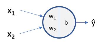
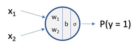
Recap - Binary Logistic Regression
Multi-Class Logistic Regression
In Multi-Class Logistic Regression, the Ouptut of the Model will be a Vector instead of a Scalar Value
Each Number in the Vector Represents the Probability of each Sample being in that Class
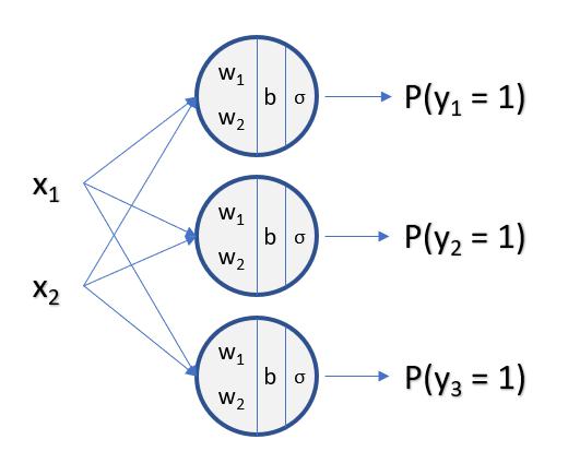
In the above scenerio of 3 Classes, the Output of the Model will be a Vector of 3 Values:
$\left[ {\begin{array}{c} P(y_{1} = 1) \\ P(y_{2} = 1) \\ P(y_{3} = 1) \end{array} } \right] $
To Output a Vector of 3 Values, We Need Three Seperate Calculations (Nodes) for Each Value
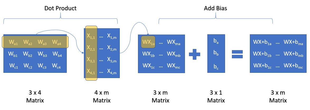
Weight Matrix:
The Weight Matrix Needs to be a (3 x 4) Matrix, or Number of Outputs (n_C) by Number of Inputs (n_F).
The Number of Rows is Number of Classes, and Number of Columns is Number of Features.
Bias Matrix:
Our Bias Matrix Needs to be a (3, 1) Matrix, or Number of Outputs (n_C) by 1.
The Number of Rows is Number of Classes, and Number of Columns is 1.
Question: Can the Sample be a Dog, a Cat, a Rat, and a Snake all at the Same Time?
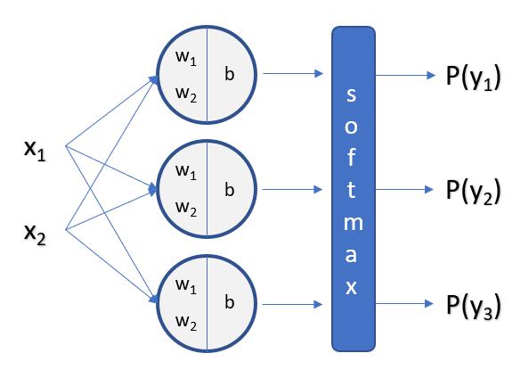
For Non-Inclusive (Exclusive) classes, We will use Softmax as our Activation Function instead of Sigmoid.
What is Softmax?
Hardmax is taking the Maximum Value of an Array and Outputting the Maximum as '1', while the rest are '0'.
$Hardmax(\left[ {\begin{array}{c} 0.1 \\ 1.2 \\ 0.5 \end{array} } \right])$ = $\left[ {\begin{array}{c} 0 \\ 1 \\ 0 \end{array} } \right]$
Softmax on the other hand, takes a 'Softer' Approach of Spreading the Values out on a Scale similar to Sigmoid.
The Highest Value will be set to a Value Closer to 1, while the Other Lower Values will be set to a Lower Value.
The Sum of All Values in the Vector for a Single Sample will add up to '1' with the below Formula:
$\sigma(z_{j}) = \frac{e^{z_{j}}}{\sum\limits^{C}_{i=1}e^{z_{i}}}$
$\sigma(Z) = \left[ {\begin{array}{c} \frac{e^{z_{1}}}{e^{z_{1}} + e^{z_{2}} + e^{z_{3}}} \\ \frac{e^{z_{2}}}{e^{z_{1}} + e^{z_{2}} + e^{z_{3}}} \\ \frac{e^{z_{3}}}{e^{z_{1}} + e^{z_{2}} + e^{z_{3}}} \end{array} } \right]$
Note that the Same Input Value might not always Output the Same Value, as the Output is Dependent on the other Input Values.
Define the Softmax Function
In [2]:
def softmax(array):
    return np.exp(array) / np.sum(np.exp(array), -1, keepdims=True)
Visualize what Softmax Does to a 2-Class Dataset
In [3]:
a = np.arange(50)/5
b = a[::-1]

c = np.vstack([a,b]).T

pd.DataFrame(c, columns=['Increasing', 'Decreasing'])
Out[3]:
In [4]:
plt.plot(softmax(c)[:,0], label='Increasing');
plt.plot(softmax(c)[:,1], label='Decreasing');
plt.xlabel('Input', fontsize=14), plt.ylabel('Output', fontsize=14)
plt.legend();

Import Iris Dataset from Sci-Kit Learn Library
In [5]:
import sklearn.datasets as datasets
import time # To Track Time
In [6]:
iris = datasets.load_iris()
Let's Check Out the Dataset
In [7]:
iris.keys()
Out[7]:
In [8]:
print("Feature Names:\n", iris['feature_names'], "\n\nLabel Names:\n", iris['target_names'])
Define Num Features (n_F) and Num Classes(n_C)
In [9]:
n_F = len(iris['feature_names'])
n_C = len(iris['target_names'])
Shape of X and Y
In [10]:
iris['data'].shape, iris['target'].shape
Out[10]:
In [11]:
df = pd.DataFrame(iris['data'], columns=iris['feature_names'])
df.head()
Out[11]:
In [12]:
X = iris['data'].T
Y_class = iris['target']
In [13]:
X.shape, Y_class.shape
Out[13]:
One-Hot Encode Labels
In [14]:
def one_hot(array, num_classes):
    new_array = np.zeros((len(array), num_classes))
    for i, val in enumerate(array):
        new_array[i, val] = 1
    return new_array
In [15]:
Y = one_hot(Y_class, n_C).T
In [16]:
Y.shape
Out[16]:
Shuffle Data
In [17]:
indices = np.arange(iris['target'].shape[0])
np.random.shuffle(indices)
In [18]:
indices
Out[18]:
In [19]:
X = X[:,indices]
Y = Y[:,indices]
Y_class = Y_class[indices]
Train Test Split
In [20]:
split_ratio = 0.2
split = int(Y.shape[1] * split_ratio)

X_train = X[:, split:]
X_val = X[:, :split]
Y_train = Y[:, split:]
Y_val = Y[:, :split]
Y_class_train = Y_class[split:]
Y_class_val = Y_class[:split]
Initialize Weights and Biases
Weights (C x F)
In [21]:
weights = np.random.randn(n_C, n_F) # Num Classes x Num Features
In [22]:
weights
Out[22]:
Biases (C x 1)
In [23]:
biases = np.zeros((n_C, 1))
In [24]:
biases
Out[24]:
Define Model
In [25]:
# Activation Function
def softmax(x):
    return np.exp(x)/sum(np.exp(x))
In [26]:
# Model
def model(biases, weights, X):
    return softmax(biases + np.dot(weights, X))
Test the Model to Check the Shape of the Output - Expected: C x M
In [27]:
model(biases, weights, X_train).shape
Out[27]:
Define Cost Function
In [28]:
def cost(prediction, Y, epsilon=1e-10):
    error = np.sum((Y * np.log(prediction + epsilon)) + ((1 - Y) * np.log(1 - prediction + epsilon)), -1)/Y.shape[1]
    return - np.sum(error)
Define Training Algorithm
In [29]:
def train(X, Y, biases, weights, epochs=1, learning_rate=1e-2, iterations=1):

    for epoch in range(epochs):
        start = time.time()
        for iteration in range(iterations):
            # Forward Pass
            pred = model(biases, weights, X)

            # Calculate Loss
            loss = cost(pred, Y)

            # Calculate Gradients
            db = np.sum((pred - Y), -1, keepdims=True) / Y.shape[1]
            dw = np.dot((pred - Y), X.T) / Y.shape[1]

            # Calculate Accuracy
            class_pred = np.argmax(pred, 0)
            class_y = np.argmax(Y, 0)
            acc = np.sum(class_pred == class_y)/Y.shape[1]

            # Update Biases and Weights
            biases -= (learning_rate * db)
            weights -= (learning_rate * dw)

        print('Epoch {}:'.format(epoch+1))
        print('Loss: {:.2f} | Accuracy: {:.2f}%\nTime Taken: {:.2f}s\n'.format(loss, acc*100, time.time()-start))

    return biases, weights
Define Function for Predicting
In [30]:
def predict(X, Y, biases, weights):
    # Forward Pass
    pred = model(biases, weights, X)

    # Calculate Accuracy
    class_pred = np.argmax(pred, 0)
    class_y = np.argmax(Y, 0)
    acc = np.sum(class_pred == class_y)/Y.shape[1]

    return acc, pred
Training The Parameters for 20 x 100 Iterations
In [31]:
biases, weights = train(X_train, Y_train, biases, weights, epochs=20, iterations=100)
In [32]:
acc, _ = predict(X_val, Y_val, biases, weights)

print('Accuracy of Prediction on Validation Data: {:.2f}%'.format(acc*100))
Sci-Kit Learn is a Powerful Python Library that has Many Built-In Machine Learning Algorithms
Import Sklearn's Logistic Regression Object from sklearn.linear_model
In [33]:
from sklearn.linear_model import LogisticRegression
Instantiate the Logistic Regression Object
In [34]:
model = LogisticRegression(solver='liblinear', multi_class='ovr', verbose=1)
Fit Model to Data
In [35]:
model.fit(X_train.T, Y_class_train)
Out[35]:
Evaluate Score of Fitted Model
In [36]:
# Training Set
model.score(X_train.T, Y_class_train)
Out[36]:
In [37]:
# Validation Set
model.score(X_val.T, Y_class_val)
Out[37]:
Note: When passing Labels(Y) into Sci-kit Learn, one-hot encoding is not required
Evaluate Cross Entropy Loss of Fitted Model
In [38]:
skpred_t = model.predict_proba(X_train.T)
skpred_v = model.predict_proba(X_val.T)
skpred = model.predict_proba(X.T)

epsilon = 1e-10

# Cross Entropy Loss
train_loss = - np.mean((Y_train.T * np.log(skpred_t + epsilon)) + ((1-Y_train.T) * np.log(1-skpred_t + epsilon)))
val_loss = - np.mean((Y_val.T * np.log(skpred_v + epsilon)) + ((1-Y_val.T) * np.log(1-skpred_v + epsilon)))
total_loss = - np.mean((Y.T * np.log(skpred + epsilon)) + ((1-Y.T) * np.log(1-skpred + epsilon)))

print('Train Set Loss: {:.4f}'.format(train_loss))
print('Validation Set Loss: {:.4f}'.format(val_loss))
print('Total Loss: {:.4f}'.format(total_loss))
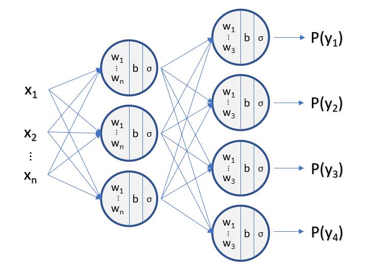
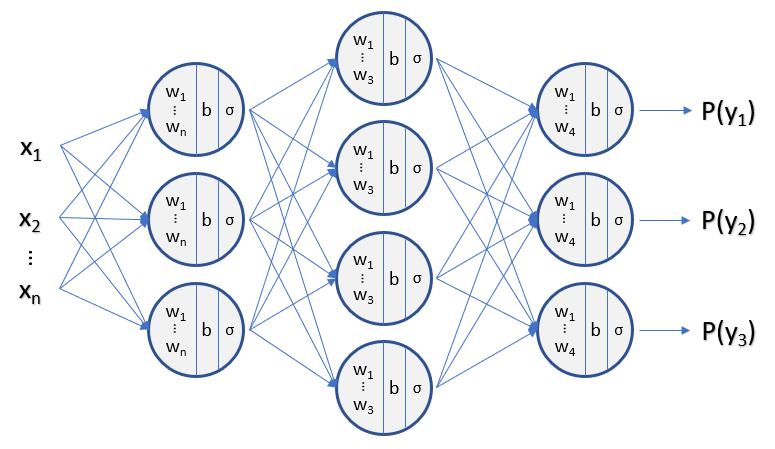
What happens if we keep stacking layers?
Naive Bayes
In [39]:
from sklearn.naive_bayes import GaussianNB
In [40]:
NB = GaussianNB()
In [41]:
NB.fit(X.T, Y_class)
Out[41]:
In [42]:
NB.score(X.T, Y_class)
Out[42]:
Decision Trees
In [43]:
from sklearn.tree import DecisionTreeClassifier
In [44]:
dec_tree = DecisionTreeClassifier()
In [45]:
dec_tree.fit(X.T, Y_class)
Out[45]:
In [46]:
dec_tree.score(X.T, Y_class)
Out[46]:
Support Vector Machines
In [47]:
from sklearn.svm import SVC
In [48]:
SVM1 = SVC(kernel='linear')
SVM2 = SVC()
In [49]:
SVM1.fit(X.T, Y_class)
SVM2.fit(X.T, Y_class)
Out[49]:
In [50]:
SVM1.score(X.T, Y_class), SVM2.score(X.T, Y_class)
Out[50]:
Ensemble Algorithms
In [51]:
from sklearn.ensemble import RandomForestClassifier
In [52]:
RFC = RandomForestClassifier()
In [53]:
RFC.fit(X.T, Y_class)
Out[53]:
In [54]:
RFC.score(X.T, Y_class)
Out[54]:
Neural Networks</h4>
In [55]:
from sklearn.neural_network import MLPClassifier
In [56]:
NN1 = MLPClassifier(max_iter=1000, hidden_layer_sizes=3)
NN2 = MLPClassifier(max_iter=1000, hidden_layer_sizes=100)
NN3 = MLPClassifier(max_iter=1000, hidden_layer_sizes=300)
In [57]:
NN1.fit(X.T, Y_class)
NN1.score(X.T, Y_class)
Out[57]:
In [58]:
NN2.fit(X.T, Y_class)
NN2.score(X.T, Y_class)
Out[58]:
In [59]:
NN3.fit(X.T, Y_class)
NN3.score(X.T, Y_class)
Out[59]:
In [60]:
NN4 = MLPClassifier(max_iter=1000, hidden_layer_sizes=(25,50,25))
In [61]:
NN4.fit(X.T, Y_class)
NN4.score(X.T, Y_class)
Out[61]:
Previous:
Next: